# Supplementary Figures
```{r setup,include=FALSE, message=FALSE, results='hide', warning=FALSE}
knitr::opts_chunk$set(cache=TRUE,echo = TRUE,warning = FALSE, message = FALSE,tinytex.verbose = TRUE, fig.align="center")
```
```{r sample-figure-data-input, echo=FALSE, results='hide',message=FALSE, fig.show="hide"}
library(pROC)
library(tidyverse)
library(data.table)
library(DT)
library(readxl)
library(parallel)
library(glmnet)
library(ggrepel)
library(grid)
library(GGally)
source("_libs/MethodD_function.R")
pkstwo <- function(x, tol = 1e-10) {
if (x < 1e-16) return(0)
j <- 1:100
sum <- sum((-1)^(j - 1) * exp(-2 * (j^2) * (x^2)))
return(2 * sum)
}
source("_libs/graphic.R")
#data
#NPXZ #POPSID+Comparator+proteins+Y #12wk:POPSID+Comparator+proteins+Roche_PlGF+Roche_PAPP_A+Roche_AFP+Roche_hCGbeta+Y+(case_type for PE_and_FGR all GAs)
#NPX #POPSID+proteins+Y
load("Rdata/dl.npxz5.Roche.ISM2.RData")
#NPX#POPSID+proteins+Y
load("Rdata/dl.npx.ISM2.RData")
#pops2 on NPXZ #POPSID+proteins+Y+(case_type for PE_and_FGR all GAs)
load("Rdata/dl.npxz5.pops2.ISM2.RData")
#data
load("Rdata/dt.olinkID.RData")#olink assays
load("Rdata/dl.npx.GA.RData")
load("Rdata/dl.npxz.GA.RData")
load("Rdata/dl.npxz.RData")
for (condition in names(dl.npxz5.pops2.ISM2)) {
for (time_point in names(dl.npxz5.pops2.ISM2[[condition]])) {
df <- dl.npxz5.pops2.ISM2[[condition]][[time_point]]
colnames(df)[ncol(df)] <- "y"
dl.npxz5.pops2.ISM2[[condition]][[time_point]] <- df}}
#load the phenotype data
phenotypes_pops_n923_anonymised <- read_excel("data/phenotypes_pops_n923_anonymised.xlsx")
#########composite data
#pops on npxz #POPSID+Comparator+proteins+Roche_PlGF+Roche_PAPP_A+Roche_AFP+Roche_hCGbeta+Y
dl.npxz5.Roche.pops.composite.12wk<- read_excel("data/dl.npxz5.Roche.pops.composite.12wk.xlsx")
##########apply winsorization at -5/5 for five biomarkers (Roche_PlGF+Roche_PAPP_A+Roche_AFP+Roche_hCGbeta)
# Vector of biomarker names to winsorize
biomarkers <- c("Roche_PlGF", "Roche_PAPP_A", "Roche_AFP", "Roche_hCGbeta")
# Count values > 5 and < -5 for each biomarker
sapply(dl.npxz5.Roche.pops.composite.12wk[biomarkers], function(x) {
gt_5 <- sum(x > 5, na.rm = TRUE)
lt_neg5 <- sum(x < -5, na.rm = TRUE)
c(`>5` = gt_5, `<-5` = lt_neg5)})
# Apply winsorization at ±5
dl.npxz5.Roche.pops.composite.12wk[biomarkers] <- lapply(
dl.npxz5.Roche.pops.composite.12wk[biomarkers],
function(x) pmax(pmin(x, 5), -5))
#pops2 on npxz #POPSID+proteins+Y
dl.npxz5.pops2.composite.12wk<- read_excel("data/dl.npxz5.pops2.composite.12wk.xlsx")
##20wk pops on npxz #POPSID+Comparator+proteins+Y
dl.npxz5.Roche.pops.composite.20wk<- read_excel("data/dl.npxz5.Roche.pops.composite.20wk.xlsx")
##28wk pops on npxz #POPSID+Comparator+proteins+Y
dl.npxz5.Roche.pops.composite.28wk<- read_excel("data/dl.npxz5.Roche.pops.composite.28wk.xlsx")
##36wk pops on npxz #POPSID+Comparator+proteins+Y
dl.npxz5.Roche.pops.composite.36wk<- read_excel("data/dl.npxz5.Roche.pops.composite.36wk.xlsx")
UtA_PI_Age_BMI_Roche_pops_12wk_com<- read_excel("data/POPS_12wk_ISM2_PE_FGR_4cat_com_UtA_PI_Age_BMI_Roche_n465.xlsx")
```
## SI Fig 1
### Histogram (NPXZ)
```{r function_histogream_V, message=FALSE, warning=FALSE}
#histogram of t test P
#POPSID+proteins+y
perform_histogram_analysis <- function(data, SIZE, group_var, P_text, axis_number, axis_size, title_size, pvalue_cutoff = 0.05, binwidth = 0.02) {
  data <- data[,-1] #proteins+y
  # Check if 'y' column exists
  if (!"y" %in% colnames(data)) {
    stop("The dataset does not contain a column named 'y'.")
  }
  # Create a matrix to store p-values and t-test statistics
  pvalue_results = matrix(rep(0, (dim(data)[2] - 1) * 2), ncol = 2)
  rownames(pvalue_results) = colnames(data)[1:(dim(data)[2] - 1)]
  colnames(pvalue_results) = c("P", "ttest")
  # Perform t-tests for each column
  for (i in 1:(dim(data)[2] - 1)) {
    pvalue_results[i, 1] = t.test(data[, i][which(data$y == 1)],
                                  data[, i][which(data$y == 0)],
                                  alternative = "two.sided", var.equal = FALSE)$p.value
    pvalue_results[i, 2] = t.test(data[, i][which(data$y == 1)],
                                  data[, i][which(data$y == 0)],
                                  alternative = "two.sided", var.equal = FALSE)$statistic  }
  # Convert results to data frame
  pvalue_results_df <- data.frame(pvalue_results)
  # Perform Kolmogorov-Smirnov test on p-values
  ks_test=ks.test(pvalue_results_df$P,"punif")
  D <- ks_test$statistic # KS test statistic
  n <- length(pvalue_results_df$P)
  # Compute the p-value
  P_input <- pkstwo(sqrt(n) * D)
  cat("KS test P-value:", P_input, "\n")
  # Count the significant p-values (less than pvalue_cutoff)
  significant_p_count <- length(which(pvalue_results_df$P < pvalue_cutoff))
  cat("Number of records with P < 0.05:", significant_p_count, "\n")
  if (anyDuplicated(pvalue_results_df$P) > 0) {
    warning("Ties detected in P values. KS test results may be affected.")
  }
  y_max <- max(table(cut(pvalue_results_df$P, breaks = 50))) +
         max(table(cut(pvalue_results_df$P, breaks = 50))) * 0.05
ggplot(pvalue_results_df, aes(x = P)) +
  geom_histogram(
    binwidth = binwidth,
    fill = "steelblue2",
    color = "black",
    breaks = seq(0, 1, by = binwidth)
  ) +
  labs(x = "P value", y = "Frequency",
       title = paste0(group_var)) +
  annotate("text",
           x = 0.5,  y = 0.9 * y_max,
           label = bquote(p ~ "=" ~.(sub("^(.*)e.*", "\\1", format(P_input, scientific = TRUE, digits = 3))) ~ "x" ~ 10^{.(as.integer(sub(".*e\\+?([-+]?[0-9]+)", "\\1", format(P_input, scientific = TRUE, digits = 3))))}),
           size = P_text,
           color = "black",
           fontface = "italic") +
  scale_y_continuous(
    expand = c(0, 0),
    limits = c(0, max(table(cut(pvalue_results_df$P, breaks = 50))) +
                 max(table(cut(pvalue_results_df$P, breaks = 50))) * 0.05),
    labels = function(y) ifelse(y == 0, "0", scales::comma(y))
  ) +
  scale_x_continuous(
    expand = c(0, 0),
    limits = c(0, 1.05),
    labels = function(x) ifelse(x == 0, "0", scales::comma(x))
  ) +
  theme_Publication() +
  theme(
    panel.grid.major = element_blank(),
    panel.grid.minor = element_blank(),
    axis.title = element_text(size = axis_size, face = "bold"),
    axis.text = element_text(size = axis_number),
    plot.title = element_text(size = title_size, face = "bold", hjust = 0.5),
    axis.line = element_line(color = "black"),
    plot.margin = margin(0.5, 0.5, 0.5, 0.5, "cm"),
    aspect.ratio = 1
  ) +
  coord_fixed(ratio = SIZE)
}
```
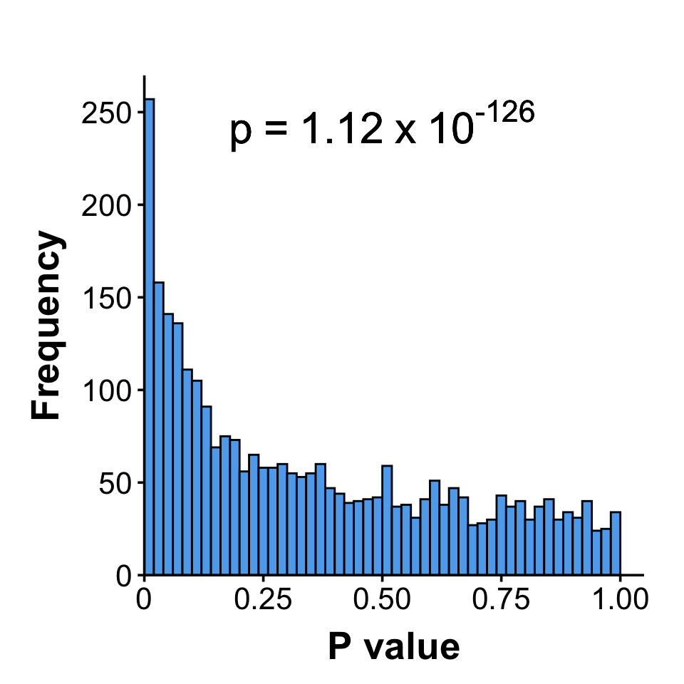
#### PE_only 12wk-Supp Fig.1a
```{r ,fig.width=5,fig.height=5,distributions_P_purePE_12wk_npxz-function_V2, echo=FALSE, message=FALSE, fig.width=5,fig.height=5}
#POPSID+proteins+y
h1=perform_histogram_analysis(data.frame(dl.npxz5.Roche.ISM2$PE_pure$`12wk`%>%dplyr::select(-c(Comparator,Roche_PlGF,Roche_PAPP_A,Roche_AFP,Roche_hCGbeta))),SIZE=1," ", P_text=8,axis_number=16, axis_size=20,title_size=20)
print(h1)
```
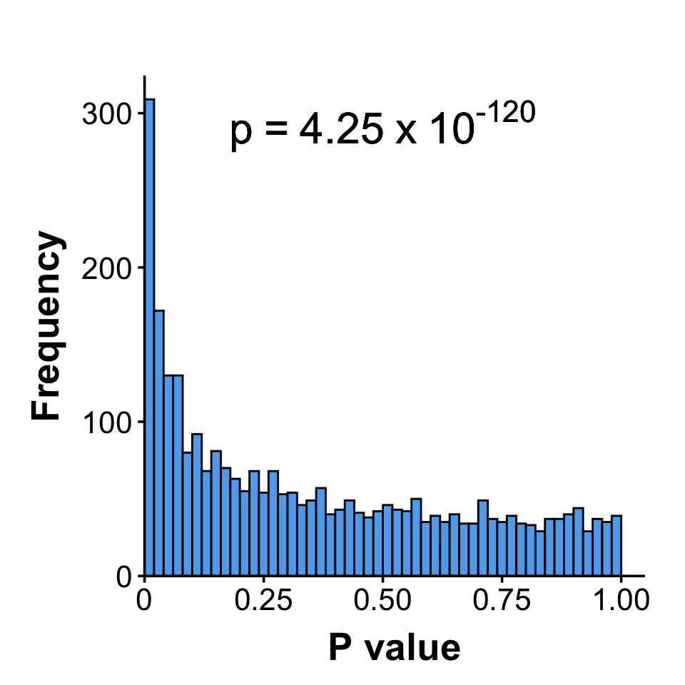
#### FGR_only 12wk-Supp Fig.1b
```{r ,fig.width=5,fig.height=5,distributions_P_pureFGR_12wk_npxz-function_V2, echo=FALSE, message=FALSE, fig.width=5,fig.height=5}
#POPSID+proteins+y
h2=perform_histogram_analysis(data.frame(dl.npxz5.Roche.ISM2$FGR_pure$`12wk`%>%dplyr::select(-c(Comparator,Roche_PlGF,Roche_PAPP_A,Roche_AFP,Roche_hCGbeta))),SIZE=1," ", P_text=8, axis_number=16, axis_size=20,title_size=20)
print(h2)
```
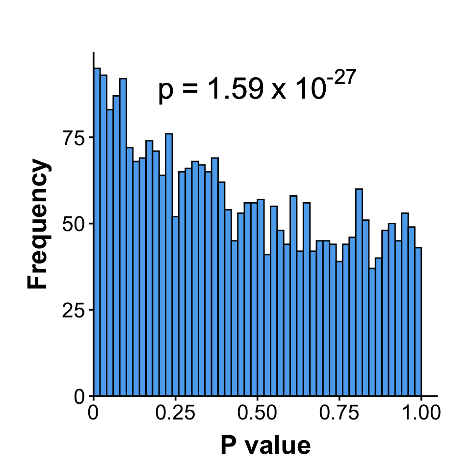
#### PE_with_FGR 12wk-Supp Fig.1c
```{r ,fig.width=5,fig.height=5,distributions_P_PE_FGR_12wk_npxz-function_V2, echo=FALSE, message=FALSE, fig.width=5,fig.height=5}
#POPSID+proteins+y
h3=perform_histogram_analysis(data.frame(dl.npxz5.Roche.ISM2$PE_and_FGR$`12wk`%>%dplyr::select(-c(Comparator,Roche_PlGF,Roche_PAPP_A,Roche_AFP,Roche_hCGbeta,case_type))),SIZE=1," ", P_text=8, axis_number=16, axis_size=20,title_size=20)
print(h3)
```
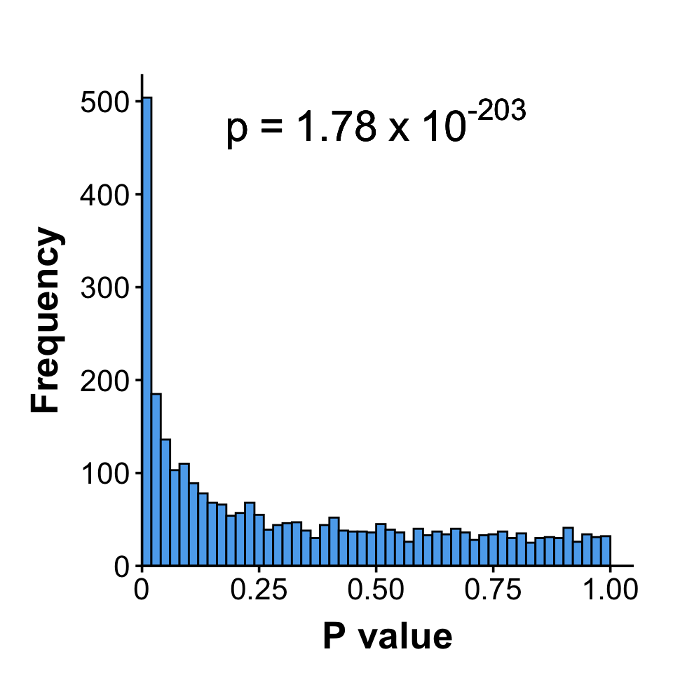
#### Composite 12wk-Supp Fig.1d
```{r ,fig.width=5,fig.height=5,distributions_P_composite_R_12wk_npxz-function_V2, echo=FALSE, message=FALSE, fig.width=5,fig.height=5}
#POPSID+proteins+y
h4=perform_histogram_analysis(data.frame(dl.npxz5.Roche.pops.composite.12wk%>%dplyr::select(-c( Comparator,Roche_PlGF,Roche_PAPP_A,Roche_AFP,Roche_hCGbeta))),SIZE=1," ", P_text=8,axis_number=16, axis_size=20,title_size=20)
print(h4)
```
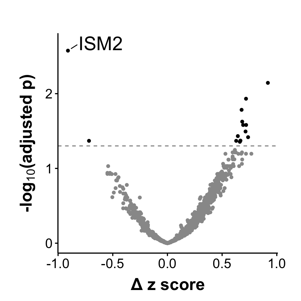
## SI Fig 2:Volcano plot for the composite outcome in the POPS2 validation cohort
## Composite 12wk NPXZ (logistic P)-Fig.d
```{r ,fig.width=5,fig.height=5,volcano_Composite_12wk_npxz-function_v2-pops2, echo=FALSE, message=FALSE, fig.width=5,fig.height=5}
#POPSID+proteins+y
create_volcano_plot(dataset =dl.npxz5.pops2.composite.12wk,SIZE=1, "Δ z score"," ",test_type = "logistic", label_size=8,axis_number=16,axis_size=20,title_size=20,box.pad=0.1,point.pad=0.5,nudge.y=0.1,nudge.x=0.2,output_file = NULL) #npx
```
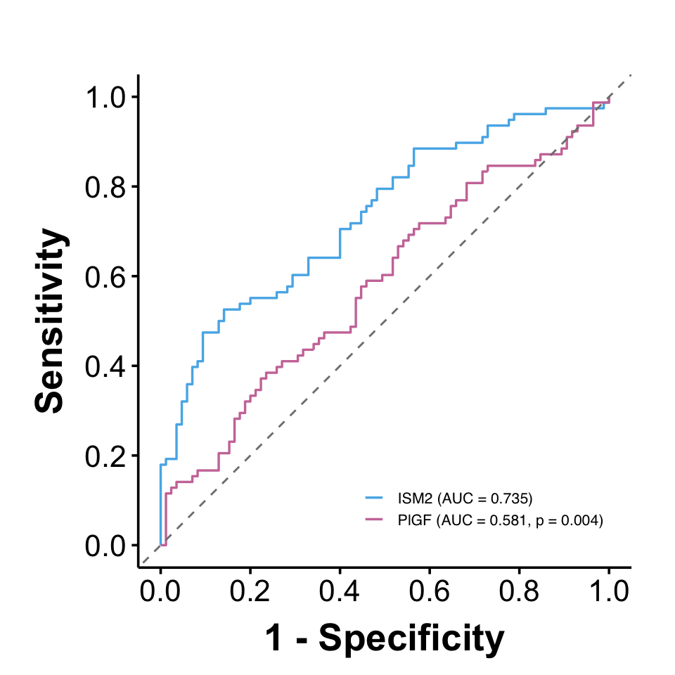
## SI Fig 3: ROC curve plots of ISM2 and PlGF in the POPS2 validation cohort
POPS2 ISM2 vs PlGF
```{r ,fig.width=5,fig.height=5,ISM2_PGF_ROC_fourinone_POPS2, message=FALSE, warning=FALSE}
plot_roc_V3 <- function(data, protein_col, plgf_col, outcome_col, title) {
  # Define colors
  condition_colors <- c(
    "ISM2" = "#56B4E9",
    "PlGF" = "#CC79A7"  )
  df <- data %>%
    dplyr::select(all_of(c(protein_col, plgf_col, outcome_col))) %>%
    dplyr::rename(y = all_of(outcome_col)) %>%
    drop_na()
  # Fit models
  fit_ism2 <- glm(y ~ ., data = df[, c("y", protein_col)], family = binomial)
  fit_plgf <- glm(y ~ ., data = df[, c("y", plgf_col)], family = binomial)
  # Predicted probabilities
  df$pred_ism2 <- fitted(fit_ism2)
  df$pred_plgf <- fitted(fit_plgf)
  # ROC objects
  roc_ism2 <- roc(df$y, df$pred_ism2, quiet = TRUE)
  roc_plgf <- roc(df$y, df$pred_plgf, quiet = TRUE)
  # AUCs
  auc_ism2 <- as.numeric(auc(roc_ism2))
  auc_plgf <- as.numeric(auc(roc_plgf))
  # DeLong test
  delong_p <- roc.test(roc_ism2, roc_plgf, method = "delong")$p.value
  # Labels
  label_ism2 <- sprintf("ISM2 (AUC = %.3f)", auc_ism2)
  label_plgf <- sprintf("PlGF (AUC = %.3f, p = %.3f)", auc_plgf, delong_p)
  roc_df <- rbind(
    data.frame(
      Specificity = roc_ism2$specificities,
      Sensitivity = roc_ism2$sensitivities,
      Protein = "ISM2",
      Label = label_ism2    ),
    data.frame(
      Specificity = roc_plgf$specificities,
      Sensitivity = roc_plgf$sensitivities,
      Protein = "PlGF",
      Label = label_plgf    )  )
  roc_df <- roc_df %>%
    dplyr::distinct(Protein, Specificity, Sensitivity, .keep_all = TRUE) %>%
    dplyr::arrange(Protein, Specificity, Sensitivity)
  p <- ggplot(roc_df,
              aes(x = 1 - Specificity,
                  y = Sensitivity,
                  color = Protein,
                  linetype = Protein)) +
    geom_step(size = 0.6, direction = "hv") +
    geom_abline(slope = 1, intercept = 0,
                linetype = "dashed", color = "gray50") +
    labs(title = title,
         x = "1 - Specificity",
         y = "Sensitivity") +
    scale_x_continuous(limits = c(0, 1), breaks = seq(0, 1, 0.2)) +
    scale_y_continuous(limits = c(0, 1), breaks = seq(0, 1, 0.2)) +
    scale_color_manual(values = condition_colors,
                       labels = c(label_ism2, label_plgf)) +
    scale_linetype_manual(values = c("ISM2" = "solid", "PlGF" = "solid"),
                          labels = c(label_ism2, label_plgf)) +
    theme_Publication() +
    theme(
      legend.position = c(0.7, 0.12), #legend.position = "none",
      legend.title = element_blank(),
      legend.text = element_text(size = 8),
      legend.key.size = unit(0.8, "lines"),
      panel.grid.major = element_blank(),
      panel.grid.minor = element_blank(),
      axis.line = element_line(colour = "black"),
      axis.title = element_text(face = "bold", size = 20),
      axis.text = element_text(size = 16),
      plot.title = element_text(size = 20, face = "bold", hjust = 0.5),
      plot.margin = margin(0.5, 0.5, 0.5, 0.5, "cm"),
      aspect.ratio = 1
    ) +
    coord_fixed(ratio = 1)
  return(list(
    plot = p,
    roc_data = roc_df,
    auc = data.frame(
      Protein = c("ISM2", "PlGF"),
      AUC = c(auc_ism2, auc_plgf)
    ),
    delong_p = delong_p
  ))
}
#composite
df_POPS2_com <- dl.npxz5.pops2.composite.12wk%>%
  dplyr::select(c("ISM2","PGF","y"))
res_pops2 <- plot_roc_V3(
  data = df_POPS2_com,
  protein_col = "ISM2",
  plgf_col = "PGF",
  outcome_col = "y",
  title = " " #"POPS2 Composite Outcome"
)
res_pops2$plot
```
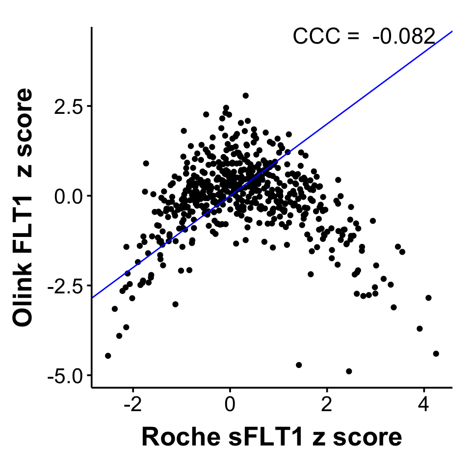
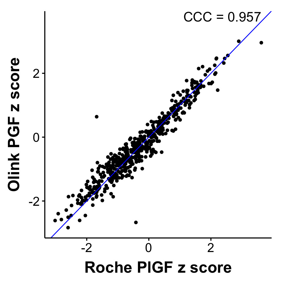
## SI Fig 7:Scatter plot of Roche values vs Olink values
Here we get the plots for the whole population – i.e. all PE, FGR and controls
```{r echo=FALSE, results='hide',message=FALSE}
if(TRUE){
dt.olinkID[Assay %in% dt.olinkID[,.N,Assay][N>1]$Assay]
dt.olinkID[Assay %in% dt.olinkID[,.N,Assay][N>1]$Assay, Assay:=paste(Assay,Panel,sep=".")]
dt.olinkID[grepl("LMOD1\\.",Assay)|grepl("SCRIB\\.",Assay)|grepl("IDO1\\.",Assay)|grepl("TNF\\.",Assay)| grepl("IL6\\.",Assay)|grepl("CXCL8\\.",Assay)]
mat.olinkID<-dt.olinkID %>% as.matrix(rownames="OlinkID")
}
Zscore4=dl.npxz.GA$`36wk`
for (l in 2:(dim(Zscore4)[2])){
colnames(Zscore4)[l]=dt.olinkID$Assay[dt.olinkID$OlinkID==colnames(Zscore4)[l]]}
#################step 1
#extract popsid from term pe
id.pe=dl.npxz$`term-PE`$`36wk`$POPSID
#extract popsid from term fgr
id.fgr=dl.npxz$`term-FGR`$`36wk`$POPSID
#id only for term PE and FGR
id=base::union(id.pe,id.fgr)
#################step 2
# Extract rows with specified POPSID values
Zscore4 <- Zscore4[Zscore4$POPSID %in% id, ]
#extract POPSID, PGF and FLT1
Zscore4 <-cbind(Zscore4$POPSID, Zscore4$PGF, Zscore4$FLT1)
colnames(Zscore4)=c("POPSID", "PGF", "FLT1")
#################step 3
#extract POPSID, comparator, Roche_PlGF, and Roche_sFLT1
outcome=data.frame(phenotypes_pops_n923_anonymised%>%dplyr::select(c("POPSID", "log2PlGF4Z", "log2sFlt_14Z")) )
outcome <- outcome[outcome$POPSID %in% id, ]
colnames(outcome)=c("POPSID", "Roche_PlGF","Roche_sFLT1")
Zscore4<-merge(Zscore4, outcome, by = c('POPSID'), all = TRUE)
```
### SI Fig 7a
```{r fig.width=5,fig.height=5,message=FALSE, warning=FALSE}
Zscore=as.data.frame(Zscore4 %>% select(c("Roche_sFLT1","FLT1")) )
Zscore=Zscore%>%drop_na()
data <- data.frame(
  Roche_sFLT1 = Zscore$Roche_sFLT1,
  Olink_FLT1 =  Zscore$FLT1)
# For calculating CCC
library(epiR)
# Calculate CCC
ccc_value <- epi.ccc(data$Roche_sFLT1, data$Olink_FLT1) #ccc_value$rho.c
# Create the scatter plot
ggplot(data, aes(x = Roche_sFLT1, y = Olink_FLT1)) +#case_control
  geom_point() +  # Add points
  geom_abline(intercept = 0, slope = 1, linetype = "solid", color = "blue") +
  xlab("Roche sFLT1 z score") +
  ylab("Olink FLT1  z score") +
  annotate("text", x = max(data$Roche_sFLT1), y = max(data$Roche_sFLT1), label = paste("CCC = ", round(ccc_value$rho.c, 3))[1], color = "black", hjust = 1, vjust = 0,size=6)+
  theme_Publication() +
    theme( legend.position = "none",
     panel.grid.major = element_blank(),
    panel.grid.minor = element_blank(),
    legend.title = element_blank(),
    axis.line = element_line(colour = "black"),
    axis.title = element_text(face = "bold", size = 20),
    axis.text = element_text(size = 16),
    plot.title = element_text(size = 20, face = "bold", hjust = 0.5),
    plot.margin = margin(0.5, 0.5, 0.5, 0.5, "cm"),
    ) +  coord_fixed(ratio = 1) +   theme(
    aspect.ratio = 1 )
```
### SI Fig 7b
```{r fig.width=5,fig.height=5,message=FALSE, warning=FALSE}
Zscore=as.data.frame(Zscore4 %>% select(c( "Roche_PlGF","PGF")) )
Zscore=Zscore%>%drop_na()
data <- data.frame(
  Roche_PlGF = Zscore$Roche_PlGF,
  Olink_PGF =  Zscore$PGF)
library(epiR)
ccc_value <- epi.ccc(data$Roche_PlGF, data$Olink_PGF)
ggplot(data, aes(x = Roche_PlGF, y = Olink_PGF)) +
  geom_point() +
  geom_abline(intercept = 0, slope = 1, linetype = "solid", color = "blue") +
  xlab("Roche PlGF z score") +
  ylab("Olink PGF z score") +
   annotate("text", x = max(data$Roche_PlGF), y = max(data$Roche_PlGF), label = paste("CCC =", round(ccc_value$rho.c, 3))[1], color = "black", hjust = 1, vjust = 0, vjust = 0,size=6)+
   theme_Publication() +
    theme( legend.position = "none",
     panel.grid.major = element_blank(),
    panel.grid.minor = element_blank(),
    legend.title = element_blank(),
    axis.line = element_line(colour = "black"),
    axis.title = element_text(face = "bold", size = 20),
    axis.text = element_text(size = 16),
    plot.title = element_text(size = 20, face = "bold", hjust = 0.5),
    plot.margin = margin(0.5, 0.5, 0.5, 0.5, "cm"),
    ) +  coord_fixed(ratio = 1) +   theme( aspect.ratio = 1   )
#Abbreviations: CCC denotes Concordance Correlation Coefficient
```