4 20 Machine Learning Methods
A number of statistical and machine learning methods are used to build 20 models.
4.1 Adaptive LOOCV Lasso
Here we use Adaptive Lasso (method 1) with leave-one-out cross-validation (LOOCV), employing the lambda.1se option based on the argument of preferring a more parsimonious model.
Code
if (file.exists(paste0("Rdata/pops_com_12wkLOOCV_adaptive.RData"))) {
#POPS composite 12wk
load("Rdata/pops_com_12wkLOOCV_adaptive.RData")
# Extract the coefficients at lambda.1se and lambda.min
coef_1se <- coef(lasso.fit, s = lasso.fit$lambda.1se)
# Find the names of non-zero coefficients
nonzero_1se <- sort(names(coef_1se[which(coef_1se != 0),][-1]))
#AUC
data <- dl.npxz5.Roche.pops.composite.12wk%>%dplyr::select(c(all_of(nonzero_1se),"y") )
model <- glm(y~. , data =data, family = binomial) #model selection
AUC=ci.auc(data$y, stats::predict(model, newdata = data, type = "response"))[2]
#CI
#ci.auc(data$y, stats::predict(model, newdata = data, type = "response"))
#LPOCV
LPOCV=get_LPOCV(data%>%mutate(y=factor(y, levels = c(0,1),labels=c("control", "case") ) ))
cat("POPS Composite 12wk: \n", "Optimal number is:", nSelectionsLOOCV.deviance.1se,
    "\n","LPOCV:", LPOCV/100,
    "\n","AUC:", AUC,
    "\n","CI:", c(ci.auc(data$y, stats::predict(model, newdata = data, type = "response"))[1],ci.auc(data$y, stats::predict(model, newdata = data, type = "response"))[3]),
    "\n","Proteins with non-zero coefficients at lambda.1se from LOOCV:\n", nonzero_1se, "\n")
adaptiveLaTrain=c(AUC,ci.auc(data$y, stats::predict(model, newdata = data, type = "response"))[1],ci.auc(data$y, stats::predict(model, newdata = data, type = "response"))[3])
} else {
f <- function(start_time) {
  start_time <- as.POSIXct(start_time)
  dt <- difftime(Sys.time(), start_time, units="secs")
  format(.POSIXct(dt,tz="GMT"), "%H:%M:%S")
}
#########composite data
#pops on npxz #POPSID+Comparator+proteins+Roche_PlGF+Roche_PAPP_A+Roche_AFP+Roche_hCGbeta+y
dl.npxz5.Roche.pops.composite.12wk<- read_excel("data/dl.npxz5.Roche.pops.composite.12wk.xlsx")
#pops2 on npxz #POPSID+proteins+y
dl.npxz5.pops2.composite.12wk<- read_excel("data/dl.npxz5.pops2.composite.12wk.xlsx")
Cuurent_E3072_batch <- read_excel("data/Cuurent E3072 batch.xlsx")
####################################################################################PEs_DN_Term 36wk:
#pre selection
{time1<-Sys.time()
    pops.com.12wk <-data.frame(dl.npxz5.Roche.pops.composite.12wk%>%dplyr::select(-c(POPSID, Comparator,Roche_PlGF,Roche_PAPP_A,Roche_AFP,Roche_hCGbeta)))
    ######################pre selection
    DAPs <- find_DEP(pops.com.12wk,mc.cores=12,pvalue=0.05)
    #for LASSO
    all.DAP=pops.com.12wk%>%
      dplyr::select(base::setdiff(DAPs$feature,Cuurent_E3072_batch$Assay),"y")%>%
      dplyr::select(-c("Roche_sFLT1"))
    set.seed(333)
    ## Perform ridge regression with CV
    ridge_cv <- cv.glmnet(
      x=as.matrix(all.DAP %>%dplyr::select(-c("y"))),
      y=all.DAP$y,
      family="binomial",
      type.measure = "deviance",
      alpha=0,
      keep=T,
      nfolds = nrow(all.DAP),
      grouped = FALSE)
    (best_ridge_coef <- coef(ridge_cv, s = ridge_cv$lambda.1se))
    best_ridge_coef  <- as.numeric(best_ridge_coef)[-1]
    set.seed(333)
    lasso.fit=cv.glmnet(
      x=as.matrix(all.DAP %>%dplyr::select(-c("y"))),
      y=all.DAP$y,
      family="binomial",
      type.measure = "deviance",
      alpha=1,
      keep=T,
      nfolds = nrow(all.DAP),
      grouped = FALSE,
      penalty.factor = 1 / abs(best_ridge_coef))
    nSelectionsLOOCV.deviance.1se <- lasso.fit$nzero[lasso.fit$lambda
                                                     == lasso.fit$lambda.1se]
    nSelectionsLOOCV.deviance.min <- lasso.fit$nzero[lasso.fit$lambda
                                                     == lasso.fit$lambda.min]
    save(file = paste0("Rdata/pops_com_12wkLOOCV_adaptive.RData"), lasso.fit,
         nSelectionsLOOCV.deviance.1se,
         nSelectionsLOOCV.deviance.min)
f(time1)}
}
POPS Composite 12wk:
Optimal number is: 26
LPOCV: 0.5013898
AUC: 0.8675833
CI: 0.8356062 0.8995604
Proteins with non-zero coefficients at lambda.1se from LOOCV:
AGRP ANXA2 CCL25 CD300E CETN2 CHMP6 CSH1 DDX39A FCRL2 GPIHBP1 HMOX1 HSD17B3 IDO1.Cardiometabolic_II IFIT3 IL1R2 ISM2 LATS1 NOS2 NTF3 PDZD2 PLA2G1B PLIN1 PLXNB3 UHRF2 VASH1 ZP4 4.2 LASSO
Code
#FDR
#POPSID+proteins+y or proteins+y
pops.com.12wk <-data.frame(dl.npxz5.Roche.pops.composite.12wk%>%dplyr::select(-c(POPSID, Comparator,Roche_PlGF,Roche_PAPP_A,Roche_AFP,Roche_hCGbeta)))
######################pre selection
DAPs <- find_DEP(pops.com.12wk,mc.cores=12,pvalue=0.05)
datatable(DAPs, rownames = F,caption = "DAPs of POPS composite at week 12",
          options = list(
  scrollX = TRUE,
  scrollCollapse = TRUE,
   order = list(1, 'desc')
)) %>%
  formatRound(c( "auc", "auc_lo", "auc_hi"), digits = 4)# include Roche_sFLT1
Code
methodD.df <- data.frame(
  No =as.character(1:10),
  Best_metabolites_PE = unlist(lapply(
    Lasso_sub(pops.com.12wk.DAP,maxNumberOfSelections=10),
    paste, sep = ";", collapse = ";")))
protein_pops_com_12wk=Lasso_sub(pops.com.12wk.DAP,maxNumberOfSelections=10)
datatable(methodD.df, rownames = FALSE,colnames = c("NO",  "Best  proteins"),caption = "Summary of selected  proteins from LASSO based on whole dataset for composite POPS at week 12",
          options = list(
            scrollX = TRUE,
            scrollY = '500px',
            scrollCollapse = TRUE,
            displayLength = 31
           ))
Lasso with top 4 proteins:
Code
data <- pops.com.12wk.DAP%>%
    dplyr::select(c(
Lasso_sub(pops.com.12wk.DAP,maxNumberOfSelections=10)[[4]], #proteins from lasso
    "y") )
  model <- glm(y~. , data =data, family = binomial)
    #AUC
  auc_pops_4=ci.auc(data$y, stats::predict(model, newdata = data, type = "response"))[2]
#LPOCV
LPOCV=get_LPOCV(data%>%mutate(y=factor(y, levels = c(0,1),labels=c("control", "case") ) ))
cat("POPS Composite 12wk: 4-predictor model \n",
    "\n","LPOCV:", LPOCV/100,
    "\n","AUC:", auc_pops_4,
    "\n","CI:", c(ci.auc(data$y, stats::predict(model, newdata = data, type = "response"))[1],ci.auc(data$y, stats::predict(model, newdata = data, type = "response"))[3]),
    "\n","4 proteins from LASSO:\n", protein_pops_com_12wk[[4]], "\n")
POPS Composite 12wk: 4-predictor model
LPOCV: 0.7610347
AUC: 0.7676129
CI: 0.7247745 0.8104513
4 proteins from LASSO:
CD300E CHMP6 CSH1 ISM2 Lasso with top 10 proteins:
Code
data <- pops.com.12wk.DAP%>%
    dplyr::select(c(
Lasso_sub(pops.com.12wk.DAP,maxNumberOfSelections=10)[[10]], #proteins from lasso
    "y") )
  model <- glm(y~. , data =data, family = binomial)
    #AUC
  auc_pops_10=ci.auc(data$y, stats::predict(model, newdata = data, type = "response"))[2]
#LPOCV
LPOCV=get_LPOCV(data%>%mutate(y=factor(y, levels = c(0,1),labels=c("control", "case") ) ))
cat("POPS Composite 12wk: 10-predictor model \n",
    "\n","LPOCV:", LPOCV/100,
    "\n","AUC:", auc_pops_10,
    "\n","CI:", c(ci.auc(data$y, stats::predict(model, newdata = data, type = "response"))[1],ci.auc(data$y, stats::predict(model, newdata = data, type = "response"))[3]),
    "\n","4 proteins from LASSO:\n", protein_pops_com_12wk[[10]], "\n")
POPS Composite 12wk: 10-predictor model
LPOCV: 0.7822333
AUC: 0.8009117
CI: 0.7617453 0.8400781
4 proteins from LASSO:
ATP6V1G1 CCL25 CD300E CHMP6 CSH1 IFIT3 ISM2 NPC2 PDZD2 UHRF2 4.3 Validation in POPS2 composite outcomes
Calculate a linear predictor for each outcome using the POPS logistic regression equations (need to use shrinkage to calculate predicted risks and for calibration plots).
Estimate the coefficients for each selected protein. These will form the linear predictor needed in the following steps. Output the linear predictor for each outcome, for example for PE: \[ \log(\text{odds}(\text{PE})) = \alpha + \beta_1 \cdot \text{PE}_{\text{protein1}} + \beta_2 \cdot \text{PE}_{\text{protein2}} + \cdots + \beta_N \cdot \text{PE}_{\text{protein}N} \] , where N = the number of proteins which from different methods above.
Calculate a uniform shrinkage factor (s) from the likelihood ratio of the fitted model (modelLR) and the effective degrees of freedom (df):
\[ s = \frac{\text{LR} - \text{df}}{\text{LR}} \] Where LR is the likelihood ratio chi-square of the model and df is the effective degrees of freedom (i.e., the number of predictors) Steyerberg (2019): Clinical Prediction Models, Chapter 13.2.1
In the following steps, apply the shrunk coefficients s x βi , i=1, …, N. For example, applying uniform shrinkage, the equation for PE is: \[ \log(\text{odds}(\text{PE})) = \alpha + s \cdot \left( \beta_1 \cdot \text{PE}_{\text{protein1}} + \beta_2 \cdot \text{PE}_{\text{protein2}} + \cdots + \beta_N \cdot \text{PE}_{\text{protein}N} \right) \]
4.3.1 Adaptive LOOCV Lasso
Selected predictors:AGRP ANXA2 CCL25 CD300E CETN2 CHMP6 CSH1 DDX39A FCRL2 GPIHBP1 HMOX1 HSD17B3 IDO1.Cardiometabolic_II IFIT3 IL1R2 ISM2 LATS1 NOS2 NTF3 PDZD2 PLA2G1B PLIN1 PLXNB3 UHRF2 VASH1 ZP4
NO. of proteins:26
Code
AUC: 0.6271493
95% CI for AUC: [0.5410119, 0.7132867]4.3.2 Lasso: 4-predictor model
Selected predictors:“CD300E” “CHMP6” “CSH1” “ISM2”
Code
AUC: 0.739819
95% CI for AUC: [0.6624047, 0.8172333]4.3.3 Lasso: 10-predictor model
Selected predictors:“ATP6V1G1” “CCL25” “CD300E” “CHMP6” “CSH1” “IFIT3” “ISM2” “NPC2” “PDZD2” “UHRF2”
Code
AUC: 0.6880845
95% CI for AUC: [0.6065543, 0.7696146]4.3.4 Lasso: 1 to 10 predictor model
Generate predictive models for 1, 2, 3… 10 proteins in POPS using Lasso
Plot the AUC for each of the models (Y axis) against the number of proteins in the model (X axis) in POPS2.
Code
auc_pops2_com_lasso10  <- calculate_auc_plot(
  data_final = dl.npxz5.Roche.pops.composite.12wk,
  protein_list = protein_pops_com_12wk,
  validation_data = dl.npxz5.pops2.composite.12wk,
  outcome_var =  "y")
datatable(auc_pops2_com_lasso10 , rownames = FALSE,colnames = c("No. of predictor model",  "AUC", "AUC_lower", "AUC_upper"),caption = "Summary of AUC from the predicted probabilities for POPS2_com using proteins from POPS_com 12wk",
          options = list(
            scrollX = TRUE,
            scrollY = '500px',
            scrollCollapse = TRUE,
            displayLength = 21
          ))%>%
  formatRound(columns = c("AUC","AUC_lo","AUC_up"), digits = 4)
Code
#AUC
line_data <- data.frame(x =auc_pops2_com_lasso10$Selections,
                        AUC=auc_pops2_com_lasso10$AUC)
melted_data <- reshape2::melt(line_data, id.vars = "x", variable.name = "measure", value.name = "Value")
maxNumberOfSelections=10
ggplot(melted_data, aes(x = x, y = Value, color =measure)) +
  geom_line(aes(col=measure),size=1.8, alpha=.8) +
  geom_point(size=2, alpha=.8,color="black") +
  geom_text(aes(label =sprintf("%.4f", Value)),  vjust = 0, hjust =0,size = 3, angle = 75) +
  labs(x="No. of predictors", y="AUC",  title ="Validation AUC plot for POPS2 composite 12wk",subtitle = "proteins from POPS composite 12wk") +
  ylim(c(0.68,0.75))+
  scale_x_continuous(
    breaks = 1:(maxNumberOfSelections),
    labels = 1:(maxNumberOfSelections),
    limits = c(0.2, maxNumberOfSelections + 1),
    expand = c(0, 0)
  ) +
  scale_x_continuous(breaks = 1:(maxNumberOfSelections+1), labels = 1:(maxNumberOfSelections+1))+
  scale_color_manual(values = c("blue")) +
  theme_bw()+
  theme(panel.grid.minor = element_blank())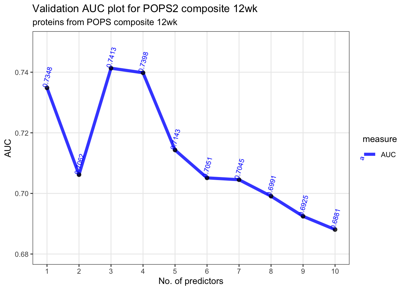
4.4 Solo predictor model (within logistic regression): ISM2
Selected predictors:“ISM2”
4.5 Other Machine Learning Methods
We perform 10-fold cross-validation using different machine learning and AI methods with the caret package in R. We train models like Random Forest (rf), Elastic net (glmnet), k-Nearest Neighbors (knn), Multivariate Adaptive Regression Splines (gcvEarth), Support Vector Machines (svmRadialCost, svmLinear2), Neural Networks (nnet, mlp, pcaNNet), LDA (lda), QDA(qda), Gaussian process classification (gaussprRadial, gaussprLinear) and XGboost (xgbTree).
Code
[1] TRUECode
[1] 163 2594.5.1 Random forest (method=“rf”)
Code
if (file.exists(paste0("data/testResults.csv"))) {
  message("File already exists. Skipping the code execution.")
} else {

if ("MOFA2" %in% .packages()) {
  detach("package:MOFA2", unload=TRUE)
}
load("trainingTest.RData")
library(randomForest)
pops.com.12wk.DAP  <- as.data.frame(pops.com.12wk.DAP)
pops2.com.12wk.dap <- as.data.frame(pops2.com.12wk.dap)
dataTrain  <- pops.com.12wk.DAP[, names(pops.com.12wk.DAP)!="y"]
classTrain <- pops.com.12wk.DAP$y
classTrain[classTrain == 0] <- "Control"
classTrain[classTrain == 1] <- "Case"
classTrain <- as.factor(classTrain)
dataTest   <- pops2.com.12wk.dap[, names(pops2.com.12wk.dap)!= "y"]
classTest  <- pops2.com.12wk.dap$y
classTest[classTest == 0] <- "Control"
classTest[classTest == 1] <- "Case"
classTest  <- as.factor(classTest)
set.seed(333)
seeds <- vector(mode = "list", length = 11)
for(i in 1:10) seeds[[i]] <- sample.int(1000, 25)
seeds[[11]] <- sample.int(1000,1)
train_ctrl <- trainControl(method="cv",
                           number = 10,
                           preProcOptions=list(cutoff=0.75),
                           seeds = seeds)
rfFit <- train(dataTrain, classTrain,
               method="rf",
               preProcess = c("corr", "nzv"),
               ntree = 200,
               tuneLength=10,
               trControl=train_ctrl)
varImpPlot(rfFit$finalModel, n.var = 10, main = "RF Variable Importance Scores")
predictionsTrain <- predict(rfFit, dataTrain, type = "prob")
roc_curveTrain <- roc(classTrain, predictionsTrain[,2])
auc_resultTrain <- auc(roc_curveTrain)
auc_ciTrain <- pROC::ci(roc_curveTrain)
predictionsTest <- predict(rfFit, dataTest, type = "prob")
roc_curveTest <- roc(classTest, predictionsTest[,2])
auc_resultTest <- auc(roc_curveTest)
auc_ciTest <- pROC::ci(roc_curveTest)
rfTrain <- auc_ciTrain[c(2, 1, 3)]
rfTest  <- auc_ciTest[c(2, 1, 3)]
}
4.5.2 Random forest with top 4 predictors (method=“rf”)
Code
if (file.exists(paste0("data/testResults.csv"))) {
  message("File already exists. Skipping the code execution.")
} else {
importanceScores <- varImp(rfFit$finalModel)
importanceScores <- importanceScores[order(importanceScores$Overall,
                                           decreasing = T),, drop= F]
selectedProteins <- rownames(importanceScores)[1:4]
set.seed(333)
seeds <- vector(mode = "list", length = 11)
for(i in 1:10) seeds[[i]] <- sample.int(1000, 25)
seeds[[11]] <- sample.int(1000,1)
train_ctrl <- trainControl(method="cv",
                           number = 10,
                           preProcOptions=list(cutoff=0.75),
                           seeds = seeds)
rftop4Fit <- train(dataTrain[,selectedProteins], classTrain,
               method="rf",
               preProcess = c("corr", "nzv"),
               ntree = 200,
               tuneLength=10,
               trControl=train_ctrl)
predictionsTrain <- predict(rftop4Fit, dataTrain, type = "prob")
roc_curveTrain <- roc(classTrain, predictionsTrain[,2])
auc_resultTrain <- auc(roc_curveTrain)
auc_ciTrain <- pROC::ci(roc_curveTrain)
predictionsTest <- predict(rftop4Fit, dataTest, type = "prob")
roc_curveTest <- roc(classTest, predictionsTest[,2])
auc_resultTest <- auc(roc_curveTest)
auc_ciTest <- pROC::ci(roc_curveTest)
rftop4Train <- auc_ciTrain[c(2, 1, 3)]
rftop4Test  <- auc_ciTest[c(2, 1, 3)]
}
4.5.3 Elastic net 1 (method=“glmnet”)
Alpha, the constant that multiplies the L1/L2 term, is the tuning parameter that decides how much we want to penalize the model. The default value is 1.0. This is called the ElasticNet mixing parameter.
Code
if (file.exists(paste0("data/testResults.csv"))) {
  message("File already exists. Skipping the code execution.")
} else {
# Elastic Net 1 (enet method)
library(caret)
library(glmnet)
library(pROC)
set.seed(333)
# Define training control for cross-validation (for model evaluation)
train_ctrl <- trainControl(method = "cv",
                           number = 10,
                           preProcOptions = list(cutoff = 0.75))
# Grid for tuning alpha and lambda (Elastic Net)
tuneGrid <- expand.grid(
  alpha = seq(0, 1, length.out = 10),  # Sequence of alpha values from 0 (Ridge) to 1 (Lasso)
  lambda = seq(0.001, 0.1, length.out = 50)  # Sequence of lambda values from 0.001 to 0.1
)
X_train <- as.matrix(dataTrain)
y_train <- as.factor(classTrain)
# Train the Elastic Net model using caret, searching over the alpha and lambda grid
enetFit <- train(
  X_train, y_train,
  method = "glmnet",
  tuneGrid = tuneGrid,
  trControl = train_ctrl,
  family = "binomial"
)
best_lambda <- enetFit$bestTune$lambda
best_alpha <- enetFit$bestTune$alpha
cat("Optimal lambda:", best_lambda, "\n")
cat("Optimal alpha:", best_alpha, "\n")
print(enetFit$bestTune)
predictionsTrain <- predict(enetFit, newdata = dataTrain, type = "prob")
roc_curveTrain <- roc(classTrain, predictionsTrain[, 2])  # ROC curve for training data
auc_resultTrain <- auc(roc_curveTrain)  # AUC result for training data
auc_ciTrain <- pROC::ci(roc_curveTrain)  # Confidence intervals for AUC
# Make predictions on test data
predictionsTest <- predict(enetFit, newdata = dataTest, type = "prob")
roc_curveTest <- roc(classTest, predictionsTest[, 2])  # ROC curve for test data
auc_resultTest <- auc(roc_curveTest)  # AUC result for test data
auc_ciTest <- pROC::ci(roc_curveTest)  # Confidence intervals for AUC
# Results: AUC and confidence intervals for both training and test data
elas1Train <- auc_ciTrain[c(2, 1, 3)]  # AUC and CI for training data
elas1Test  <- auc_ciTest[c(2, 1, 3)]   # AUC and CI for test data
cat("Training AUC (CI):", elas1Train, "\n")
cat("Test AUC (CI):", elas1Test, "\n")
}
4.5.4 Elastic net 2 (method=“glmnet”)
We get Elastic Net 2 after fitting Elastic Net 1 (we get optimal alpha from Elastic Net 1)
1.Use the optimal alpha from Elastic Net 1
2.Then tune lambda only
3.Rescale coefficients after model fitting (that’s what distinguishes Elastic Net 2 from Elastic Net 1).
Code
if (file.exists(paste0("data/testResults.csv"))) {
  message("File already exists. Skipping the code execution.")
} else {
# Elastic Net 2 (glmnet method)
set.seed(333)
train_ctrl <- trainControl(method = "cv",
                           number = 10,
                           preProcOptions = list(cutoff = 0.75))
best_alpha <- enetFit$bestTune$alpha
# Fit cv.glmnet with only lambda tuning
ela2_glmnet <- cv.glmnet(
  x = as.matrix(dataTrain),
  y = as.factor(classTrain),
  family = "binomial",
  alpha = best_alpha,
  keep = TRUE)
# Get best lambda
best_lambda <- ela2_glmnet$lambda.min
# Extract non-zero coefficients (excluding intercept)
coeff_matrix <- coef(ela2_glmnet, s = "lambda.min") %>% as.matrix()
nonzero_vars <- rownames(coeff_matrix)[which(coeff_matrix != 0)][-1]  # drop intercept
# Build formula from selected variables
formula_reduced <- as.formula(paste("classTrain ~", paste(nonzero_vars, collapse = "+")))
# Create data frame for glm model
dataTrain_glm <- data.frame(classTrain, dataTrain)
dataTest_glm <- data.frame(classTest, dataTest)
# Fit reduced logistic model using glm
glm_reduced <- glm(formula_reduced, data = dataTrain_glm, family = binomial)
#Make predictions on training data
predictionsTrain <- predict(glm_reduced, newdata = dataTrain_glm, type = "response")
roc_curveTrain <- roc(dataTrain_glm$classTrain, predictionsTrain)  # ROC curve for training data
auc_resultTrain <- auc(roc_curveTrain)  # AUC result for training data
auc_ciTrain <- pROC::ci(roc_curveTrain)  # Confidence intervals for AUC
#Make predictions on test data
predictionsTest <- predict(glm_reduced, newdata = dataTest_glm, type = "response")
roc_curveTest <- roc(dataTest_glm$classTest, predictionsTest)  # ROC curve for test data
auc_resultTest <- auc(roc_curveTest)  # AUC result for test data
auc_ciTest <- pROC::ci(roc_curveTest)  # Confidence intervals for AUC
#AUC and confidence intervals for both training and test data
elas2Train <- auc_ciTrain[c(2, 1, 3)]  # AUC, lower CI, upper CI
elas2Test  <- auc_ciTest[c(2, 1, 3)]
cat("Training AUC (CI):", round(elas2Train, 4), "\n")
cat("Test AUC (CI):", round(elas2Test, 4), "\n")
}
4.5.5 k nearest neighbour (method=“knn”)
Code
if (file.exists(paste0("data/testResults.csv"))) {
  message("File already exists. Skipping the code execution.")
} else {
set.seed(333)
train_ctrl <- trainControl(method="cv",
                           number = 10,
                           preProcOptions=list(cutoff=0.75))
knnFit <- train(dataTrain, classTrain,
               method="knn",
               preProcess = c("corr", "nzv"),
               tuneLength=30,
               trControl=train_ctrl)
predictionsTrain <- predict(knnFit, newdata = dataTrain, type = "prob")
roc_curveTrain <- roc(classTrain, predictionsTrain[,2])
auc_resultTrain <- auc(roc_curveTrain)
auc_ciTrain <- pROC::ci(roc_curveTrain)
predictionsTest <- predict(knnFit, dataTest, type = "prob")
roc_curveTest <- roc(classTest, predictionsTest[,2])
auc_resultTest <- auc(roc_curveTest)
auc_ciTest <- pROC::ci(roc_curveTest)
knnTrain <- auc_ciTrain[c(2, 1, 3)]
knnTest  <- auc_ciTest[c(2, 1, 3)]
}
4.5.6 PCA + k nearest neighbour (method=“knn”)
Code
if (file.exists(paste0("data/testResults.csv"))) {
  message("File already exists. Skipping the code execution.")
} else {
PCAtrain <- prcomp(dataTrain, center = TRUE, scale = TRUE)
plot(1:20, (PCAtrain$sdev^2)[1:20])
PCAtest  <- predict(PCAtrain, dataTest)
set.seed(333)
train_ctrl <- trainControl(method="cv",
                           number = 10,
                           preProcOptions=list(cutoff=0.75))
knnFit <- train(PCAtrain$x[,1:5], classTrain,
               method="knn",
               preProcess = c("corr", "nzv"),
               tuneLength=30,
               trControl=train_ctrl)
predictionsTrain <- predict(knnFit, newdata = PCAtrain$x[,1:5], type = "prob")
roc_curveTrain <- roc(classTrain, predictionsTrain[,2])
auc_resultTrain <- auc(roc_curveTrain)
auc_ciTrain <- pROC::ci(roc_curveTrain)
predictionsTest <- predict(knnFit, PCAtest[,1:5], type = "prob")
roc_curveTest <- roc(classTest, predictionsTest[,2])
auc_resultTest <- auc(roc_curveTest)
auc_ciTest <- pROC::ci(roc_curveTest)
knnPCA4Train <- auc_ciTrain[c(2, 1, 3)]
knnPCA4Test  <- auc_ciTest[c(2, 1, 3)]
}
4.5.7 Multivariate Adaptive Regression Splines (method=“gcvEarth”)
Code
if (file.exists(paste0("data/testResults.csv"))) {
  message("File already exists. Skipping the code execution.")
} else {
set.seed(333)
train_ctrl <- trainControl(method="cv",
                           number = 10,
                           preProcOptions=list(cutoff=0.75))
gcvEarthFit <- train(dataTrain, classTrain,
               method="gcvEarth",
               preProcess = c("corr", "nzv"),
               tuneLength=10,
               trControl=train_ctrl)
predictionsTrain <- predict(gcvEarthFit, newdata = dataTrain, type = "prob")
roc_curveTrain <- roc(classTrain, predictionsTrain[,2])
auc_resultTrain <- auc(roc_curveTrain)
auc_ciTrain <- pROC::ci(roc_curveTrain)
predictionsTest <- predict(gcvEarthFit, dataTest, type = "prob")
roc_curveTest <- roc(classTest, predictionsTest[,2])
auc_resultTest <- auc(roc_curveTest)
auc_ciTest <- pROC::ci(roc_curveTest)
gcvEarthTrain <- auc_ciTrain[c(2, 1, 3)]
gcvEarthTest  <- auc_ciTest[c(2, 1, 3)]
}
4.5.8 Support Vector Machine (Linear kernel) (method=“svmLinear2”)
Code
if (file.exists(paste0("data/testResults.csv"))) {
  message("File already exists. Skipping the code execution.")
} else {
set.seed(333)
train_ctrl <- trainControl(method="cv",
                           number = 10,
                           preProcOptions=list(cutoff=0.75),
                           classProbs=TRUE)
svmLinear2Fit <- train(dataTrain, classTrain,
               method="svmLinear2",
               preProcess = c("corr", "nzv"),
               tuneLength=10,
               trControl=train_ctrl)
predictionsTrain <- predict(svmLinear2Fit, newdata = dataTrain, type = "prob")
roc_curveTrain <- roc(classTrain, predictionsTrain[,2])
auc_resultTrain <- auc(roc_curveTrain)
auc_ciTrain <- pROC::ci(roc_curveTrain)
predictionsTest <- predict(svmLinear2Fit, dataTest, type = "prob")
roc_curveTest <- roc(classTest, predictionsTest[,2])
auc_resultTest <- auc(roc_curveTest)
auc_ciTest <- pROC::ci(roc_curveTest)
svmLinear2Train <- auc_ciTrain[c(2, 1, 3)]
svmLinear2Test  <- auc_ciTest[c(2, 1, 3)]
}
4.5.9 Neural network 2 (method=“nnet”)
Code
if (file.exists(paste0("data/testResults.csv"))) {
  message("File already exists. Skipping the code execution.")
} else {
set.seed(333)
train_ctrl <- trainControl(method="cv",
                           number = 10,
                           preProcOptions=list(cutoff=0.75))
nnetFit <- train(dataTrain, classTrain,
               method="nnet",
               preProcess = c("corr", "nzv"),
               tuneLength=10,
               trControl=train_ctrl)
predictionsTrain <- predict(nnetFit, newdata = dataTrain, type = "prob")
roc_curveTrain <- roc(classTrain, predictionsTrain[,2])
auc_resultTrain <- auc(roc_curveTrain)
auc_ciTrain <- pROC::ci(roc_curveTrain)
predictionsTest <- predict(nnetFit, dataTest, type = "prob")
roc_curveTest <- roc(classTest, predictionsTest[,2])
auc_resultTest <- auc(roc_curveTest)
auc_ciTest <- pROC::ci(roc_curveTest)
nnetTrain <- auc_ciTrain[c(2, 1, 3)]
nnetTest  <- auc_ciTest[c(2, 1, 3)]
}
4.5.10 Neural Networks with Feature Extraction (PCA + Neural Network) (method=“pcaNNet”)
Code
if (file.exists(paste0("data/testResults.csv"))) {
  message("File already exists. Skipping the code execution.")
} else {
set.seed(333)
train_ctrl <- trainControl(method="cv",
                           number = 10,
                           preProcOptions=list(cutoff=0.75))
pcaNNetFit <- train(dataTrain, classTrain,
               method="pcaNNet",
               preProcess = c("corr", "nzv"),
               tuneLength=10,
               trControl=train_ctrl)
predictionsTrain <- predict(pcaNNetFit, newdata = dataTrain, type = "prob")
roc_curveTrain <- roc(classTrain, predictionsTrain[,2])
auc_resultTrain <- auc(roc_curveTrain)
auc_ciTrain <- pROC::ci(roc_curveTrain)
predictionsTest <- predict(pcaNNetFit, dataTest, type = "prob")
roc_curveTest <- roc(classTest, predictionsTest[,2])
auc_resultTest <- auc(roc_curveTest)
auc_ciTest <- pROC::ci(roc_curveTest)
pcaNNetTrain <- auc_ciTrain[c(2, 1, 3)]
pcaNNetTest  <- auc_ciTest[c(2, 1, 3)]
}
4.5.11 Linear Discriminant Analysis (LDA) (method=“lda”)
Code
if (file.exists(paste0("data/testResults.csv"))) {
  message("File already exists. Skipping the code execution.")
} else {
set.seed(333)
train_ctrl <- trainControl(method="cv",
                           number = 10,
                           preProcOptions=list(cutoff=0.75))
ldaFit <- train(dataTrain, classTrain,
               method="lda",
               preProcess = c("corr", "nzv"),
               tuneLength=10,
               trControl=train_ctrl)
predictionsTrain <- predict(ldaFit, newdata = dataTrain, type = "prob")
roc_curveTrain <- roc(classTrain, predictionsTrain[,2])
auc_resultTrain <- auc(roc_curveTrain)
auc_ciTrain <- pROC::ci(roc_curveTrain)
predictionsTest <- predict(ldaFit, dataTest, type = "prob")
roc_curveTest <- roc(classTest, predictionsTest[,2])
auc_resultTest <- auc(roc_curveTest)
auc_ciTest <- pROC::ci(roc_curveTest)
ldaTrain <- auc_ciTrain[c(2, 1, 3)]
ldaTest  <- auc_ciTest[c(2, 1, 3)]
}
4.5.12 Quadratic Discriminant Analysis (QDA) (method=“qda”)
Code
if (file.exists(paste0("data/testResults.csv"))) {
  message("File already exists. Skipping the code execution.")
} else {
set.seed(333)
train_ctrl <- trainControl(method="cv",
                           number = 10,
                           preProcOptions=list(cutoff=0.75))
qdaFit <- train(dataTrain, classTrain,
               method="qda",
               preProcess = c("corr", "nzv"),
               tuneLength=10,
               trControl=train_ctrl)
predictionsTrain <- predict(qdaFit, newdata = dataTrain, type = "prob")
roc_curveTrain <- roc(classTrain, predictionsTrain[,2])
auc_resultTrain <- auc(roc_curveTrain)
auc_ciTrain <- pROC::ci(roc_curveTrain)
predictionsTest <- predict(qdaFit, dataTest, type = "prob")
roc_curveTest <- roc(classTest, predictionsTest[,2])
auc_resultTest <- auc(roc_curveTest)
auc_ciTest <- pROC::ci(roc_curveTest)
qdaTrain <- auc_ciTrain[c(2, 1, 3)]
qdaTest  <- auc_ciTest[c(2, 1, 3)]
}
4.5.13 Support Vector Machine (Radial kernel) (method=“svmRadialCost”)
Code
if (file.exists(paste0("data/testResults.csv"))) {
  message("File already exists. Skipping the code execution.")
} else {
library(kernlab)
set.seed(333)
train_ctrl <- trainControl(method="cv",
                           number = 10,
                           preProcOptions=list(cutoff=0.75),
                           classProbs=TRUE)
svmRadialCostFit <- train(dataTrain, classTrain,
               method="svmRadialCost",
               preProcess = c("corr", "nzv"),
               tuneLength=10,
               trControl=train_ctrl)
predictionsTrain <- predict(svmRadialCostFit, newdata = dataTrain, type = "prob")
roc_curveTrain <- roc(classTrain, predictionsTrain[,2])
auc_resultTrain <- auc(roc_curveTrain)
auc_ciTrain <- pROC::ci(roc_curveTrain)
predictionsTest <- predict(svmRadialCostFit, dataTest, type = "prob")
roc_curveTest <- roc(classTest, predictionsTest[,2])
auc_resultTest <- auc(roc_curveTest)
auc_ciTest <- pROC::ci(roc_curveTest)
svmRadialCostTrain <- auc_ciTrain[c(2, 1, 3)]
svmRadialCostTest  <- auc_ciTest[c(2, 1, 3)]
}
4.5.14 Gaussian process classification (radial kernel) (method=“gaussprRadial”)
Code
if (file.exists(paste0("data/testResults.csv"))) {
  message("File already exists. Skipping the code execution.")
} else {
set.seed(333)
train_ctrl <- trainControl(method="cv",
                           number = 10,
                           preProcOptions=list(cutoff=0.75))
gaussprRadialFit <- train(dataTrain, classTrain,
               method="gaussprRadial",
               preProcess = c("corr", "nzv"),
               tuneLength=10,
               trControl=train_ctrl)
predictionsTrain <- predict(gaussprRadialFit, newdata = dataTrain, type = "prob")
roc_curveTrain <- roc(classTrain, predictionsTrain[,2])
auc_resultTrain <- auc(roc_curveTrain)
auc_ciTrain <- pROC::ci(roc_curveTrain)
predictionsTest <- predict(gaussprRadialFit, dataTest, type = "prob")
roc_curveTest <- roc(classTest, predictionsTest[,2])
auc_resultTest <- auc(roc_curveTest)
auc_ciTest <- pROC::ci(roc_curveTest)
gaussprRadialTrain <- auc_ciTrain[c(2, 1, 3)]
gaussprRadialTest  <- auc_ciTest[c(2, 1, 3)]
}
4.5.15 Gaussian process classification (linear kernel) (method=“gaussprLinear”)
Code
if (file.exists(paste0("data/testResults.csv"))) {
  message("File already exists. Skipping the code execution.")
} else {
set.seed(333)
train_ctrl <- trainControl(method="cv",
                           number = 10,
                           preProcOptions=list(cutoff=0.75))
gaussprLinearFit <- train(dataTrain, classTrain,
               method="gaussprLinear",
               preProcess = c("corr", "nzv"),
               tuneLength=10,
               trControl=train_ctrl)
predictionsTrain <- predict(gaussprLinearFit, newdata = dataTrain, type = "prob")
roc_curveTrain <- roc(classTrain, predictionsTrain[,2])
auc_resultTrain <- auc(roc_curveTrain)
auc_ciTrain <- pROC::ci(roc_curveTrain)
predictionsTest <- predict(gaussprLinearFit, dataTest, type = "prob")
roc_curveTest <- roc(classTest, predictionsTest[,2])
auc_resultTest <- auc(roc_curveTest)
auc_ciTest <- pROC::ci(roc_curveTest)
gaussprLinearTrain <- auc_ciTrain[c(2, 1, 3)]
gaussprLinearTest  <- auc_ciTest[c(2, 1, 3)]
}
4.5.16 Neural network (method=“mlp”)
Code
if (file.exists(paste0("data/testResults.csv"))) {
  message("File already exists. Skipping the code execution.")
} else {
set.seed(333)
train_ctrl <- trainControl(method="cv",
                           number = 10,
                           preProcOptions=list(cutoff=0.75))
mlpFit <- train(dataTrain, classTrain,
               method="mlp",
               preProcess = c("corr", "nzv"),
               tuneLength=10,
               trControl=train_ctrl)
predictionsTrain <- predict(mlpFit, newdata = dataTrain, type = "prob")
roc_curveTrain <- roc(classTrain, predictionsTrain[,2])
auc_resultTrain <- auc(roc_curveTrain)
auc_ciTrain <- pROC::ci(roc_curveTrain)
predictionsTest <- predict(mlpFit, dataTest, type = "prob")
roc_curveTest <- roc(classTest, predictionsTest[,2])
auc_resultTest <- auc(roc_curveTest)
auc_ciTest <- pROC::ci(roc_curveTest)
mlpTrain <- auc_ciTrain[c(2, 1, 3)]
mlpTest  <- auc_ciTest[c(2, 1, 3)]
}
4.5.17 XGboost (method=“xgbTree”)
Code
if (file.exists(paste0("data/testResults.csv"))) {
  message("File already exists. Skipping the code execution.")
} else {
{time1<-Sys.time()
set.seed(333)
 train_ctrl <- trainControl(method="cv",
                            number = 10,
                            preProcOptions=list(cutoff=0.75),
                            classProbs = TRUE)
 xgb.grid = expand.grid(
     nrounds = 1000,
     eta = c(0.001, 0.005, 0.01, 0.02, 0.05, 0.1, 0.2, 0.3),
     max_depth = c(2, 4, 6, 8),
     gamma = c(1, 2, 3),
     subsample = c(0.5, 0.75, 1),
     min_child_weight = c(1, 2, 3),
     colsample_bytree = 1 )
 xgbTreeFit <- train(dataTrain, classTrain,
                method="xgbTree",
                preProcess = c("corr", "nzv"),
                  tuneGrid=xgb.grid,
                trControl=train_ctrl)
 predictionsTrain <- predict(xgbTreeFit, newdata = dataTrain, type = "prob")
 roc_curveTrain <- roc(classTrain, predictionsTrain[,2])
 auc_resultTrain <- auc(roc_curveTrain)
 auc_ciTrain <- pROC::ci(roc_curveTrain)
 predictionsTest <- predict(xgbTreeFit, dataTest, type = "prob")
 roc_curveTest <- roc(classTest, predictionsTest[,2])
 auc_resultTest <- auc(roc_curveTest)
 auc_ciTest <- pROC::ci(roc_curveTest)
 xgbTreeTrain <- auc_ciTrain[c(2, 1, 3)]
 xgbTreeTest  <- auc_ciTest[c(2, 1, 3)]
  f(time1)
}
}