# Main Figures
```{r setup,include=FALSE, message=FALSE, results='hide', warning=FALSE}
knitr::opts_chunk$set(cache=TRUE,echo = TRUE,warning = FALSE, message = FALSE,tinytex.verbose = TRUE, fig.align="center")
```
```{r sample-figure-data-input, echo=FALSE, results='hide',message=FALSE, fig.show="hide"}
library(pROC)
library(tidyverse)
library(data.table)
library(DT)
library(readxl)
library(parallel)
library(glmnet)
library(ggrepel)
library(grid)
library(ggbeeswarm)
source("_libs/MethodD_function.R")
source("_libs/graphic.R")
#data
load("Rdata/dt.olinkID.RData")
#NPX
load("Rdata/dl.npx.GA.RData")
#NPXZ #POPSID+Comparator+proteins+Y #12wk:POPSID+Comparator+proteins+Roche_PlGF+Roche_PAPP_A+Roche_AFP+Roche_hCGbeta+Y+(case_type for PE_and_FGR all GAs)
#NPX #POPSID+proteins+Y
load("Rdata/dl.npxz5.Roche.ISM2.RData")
#NPX#POPSID+proteins+Y
load("Rdata/dl.npx.ISM2.RData")
#pops2 on NPXZ #POPSID+proteins+Y+(case_type for PE_and_FGR all GAs)
load("Rdata/dl.npxz5.pops2.ISM2.RData")
for (condition in names(dl.npxz5.pops2.ISM2)) {
for (time_point in names(dl.npxz5.pops2.ISM2[[condition]])) {
df <- dl.npxz5.pops2.ISM2[[condition]][[time_point]]
colnames(df)[ncol(df)] <- "y"
dl.npxz5.pops2.ISM2[[condition]][[time_point]] <- df}}
#load the phenotype data
phenotypes_pops_n923_anonymised <- read_excel("data/phenotypes_pops_n923_anonymised.xlsx")
#########composite data
#pops on npxz #POPSID+Comparator+proteins+Roche_PlGF+Roche_PAPP_A+Roche_AFP+Roche_hCGbeta+Y
dl.npxz5.Roche.pops.composite.12wk<- read_excel("data/dl.npxz5.Roche.pops.composite.12wk.xlsx")
##########
biomarkers <- c("Roche_PlGF", "Roche_PAPP_A", "Roche_AFP", "Roche_hCGbeta")
sapply(dl.npxz5.Roche.pops.composite.12wk[biomarkers], function(x) {
gt_5 <- sum(x > 5, na.rm = TRUE)
lt_neg5 <- sum(x < -5, na.rm = TRUE)
c(`>5` = gt_5, `<-5` = lt_neg5)})
# Apply winsorization at ±5
dl.npxz5.Roche.pops.composite.12wk[biomarkers] <- lapply(
dl.npxz5.Roche.pops.composite.12wk[biomarkers],
function(x) pmax(pmin(x, 5), -5))
#pops2 on npxz #POPSID+proteins+Y
dl.npxz5.pops2.composite.12wk<- read_excel("data/dl.npxz5.pops2.composite.12wk.xlsx")
##20wk pops on npxz #POPSID+Comparator+proteins+Y
dl.npxz5.Roche.pops.composite.20wk<- read_excel("data/dl.npxz5.Roche.pops.composite.20wk.xlsx")
##28wk pops on npxz #POPSID+Comparator+proteins+Y
dl.npxz5.Roche.pops.composite.28wk<- read_excel("data/dl.npxz5.Roche.pops.composite.28wk.xlsx")
##36wk pops on npxz #POPSID+Comparator+proteins+Y
dl.npxz5.Roche.pops.composite.36wk<- read_excel("data/dl.npxz5.Roche.pops.composite.36wk.xlsx")
UtA_PI_Age_BMI_Roche_pops_12wk_com<- read_excel("data/POPS_12wk_ISM2_PE_FGR_4cat_com_UtA_PI_Age_BMI_Roche_n465.xlsx")
#POPS npxz:for every analyses npxz #POPSID+proteins+Y
load("Rdata/dl.npxz5.Roche.final.RData")
```
## Figure 1
### Volcano plot
```{r function_volcano_v, message=FALSE, warning=FALSE}
create_volcano_plot <- function(dataset, SIZE = 1, x_label, group_var, test_type = c("logistic", "ttest"),
                               label_size, axis_number, axis_size, title_size, box.pad, point.pad,
                               nudge.y, nudge.x) {
  ZscoreMoMs4pe <- data.frame(dataset)[,-1]
  differencePE4 <- matrix(rep(0, (dim(ZscoreMoMs4pe)[2] - 1)), ncol = 1)
  for (i in 1:(dim(ZscoreMoMs4pe)[2] - 1)) {
    differencePE4[i] <- mean(na.omit(ZscoreMoMs4pe[,i][which(ZscoreMoMs4pe$y == 1)])) -
                        mean(na.omit(ZscoreMoMs4pe[,i][which(ZscoreMoMs4pe$y == 0)]))
  }
  pvaluePE4 <- matrix(rep(0, (dim(ZscoreMoMs4pe)[2] - 1) * 2), ncol = 2)
  rownames(pvaluePE4) <- colnames(ZscoreMoMs4pe)[1:(dim(ZscoreMoMs4pe)[2] - 1)]
  colnames(pvaluePE4) <- c("P", "Test Statistic")
  for (i in 1:(dim(ZscoreMoMs4pe)[2] - 1)) {
    if (test_type == "logistic") {
      pvaluePE4[i, 1] <- coef(summary(glm(X1 ~ X2, family = "binomial",
                                         data = data.frame(cbind(ZscoreMoMs4pe$y, ZscoreMoMs4pe[, i])))))[, 'Pr(>|z|)'][2]
      pvaluePE4[i, 2] <- exp(coef(glm(X1 ~ X2, family = "binomial",
                                     data = data.frame(cbind(ZscoreMoMs4pe$y, ZscoreMoMs4pe[, i])))))[2]
    } else if (test_type == "ttest") {
      pvaluePE4[i, 1] <- t.test(ZscoreMoMs4pe[, i][which(ZscoreMoMs4pe$y == 1)],
                                ZscoreMoMs4pe[, i][which(ZscoreMoMs4pe$y == 0)],
                                alternative = "two.sided", var.equal = FALSE)$p.value
      pvaluePE4[i, 2] <- t.test(ZscoreMoMs4pe[, i][which(ZscoreMoMs4pe$y == 1)],
                                ZscoreMoMs4pe[, i][which(ZscoreMoMs4pe$y == 0)],
                                alternative = "two.sided", var.equal = FALSE)$statistic
    }
  }
  pvaluePE4 <- data.frame(pvaluePE4)
  padj.BY.PE4 <- data.frame(p.adjust(pvaluePE4$P, method = "BH"))
  DAMpe4 <- rownames(pvaluePE4)[as.numeric(rownames(padj.BY.PE4)[which(padj.BY.PE4 < 0.05)])]
  padj.BY.PE4.vol <- -log10(padj.BY.PE4)
  padj.BY.PE4.vol$protein <- rownames(pvaluePE4)
  padj.BY.PE4.vol$protein <- gsub("^NT\\.proBNP$", "NT-proBNP", padj.BY.PE4.vol$protein)
  padj.BY.PE4.vol$protein <- gsub("^HLA\\.DRA$", "HLA-DRA", padj.BY.PE4.vol$protein)
  padj.BY.PE4.vol$protein <- gsub("^HLA\\.E$", "HLA-E", padj.BY.PE4.vol$protein)
  padj.BY.PE4.vol$protein <- gsub("^ERVV\\.1$", "ERVV-1", padj.BY.PE4.vol$protein)
  padj.BY.PE4.vol$protein <- gsub("^HLA\\.A$", "HLA-A", padj.BY.PE4.vol$protein)
  padj.BY.PE4.vol$Metabolites <- as.factor(ifelse(padj.BY.PE4 < 0.05, "DAMs", "Other meta"))
  padj.BY.PE4.vol$log2FoldChange <- differencePE4
  colnames(padj.BY.PE4.vol) <- c("-log10(padj.BY.PE4)", "protein", "Metabolites", "log2FoldChange")
  padj.BY.PE4.vol <- na.omit(padj.BY.PE4.vol)
  padj.BY.PE4.vol$label <- NA
  padj.BY.PE4.vol$label[padj.BY.PE4.vol$Metabolites == "DAMs"] <-
  padj.BY.PE4.vol$protein[padj.BY.PE4.vol$Metabolites == "DAMs"]
  p <- ggplot(data = padj.BY.PE4.vol, aes(log2FoldChange, `-log10(padj.BY.PE4)`, col = Metabolites, label = label)) +
    geom_point() +
    ylab(expression(bold("-") * bold(log)[bold(10)] * bold("(adjusted p)"))) +
    geom_hline(yintercept = -log10(0.05), linetype = "dashed", col = "grey50") +
    xlab(paste0(x_label)) +
    labs(title = paste0(group_var)) +
    scale_color_manual(values = c("DAMs" = "#000000", "Other meta" = "#999999"), guide = FALSE) +
    scale_y_continuous(breaks = function(x) floor(min(x)):ceiling(max(x))) +
    geom_text_repel(
      data = subset(padj.BY.PE4.vol, protein == "ISM2"),
      aes(label = protein),
      box.padding = box.pad,
      size = label_size,
      point.padding = point.pad,
      max.overlaps = 20,
      nudge_y = nudge.y,
      nudge_x = nudge.x + 0.1,
      segment.color = 'black',
      segment.size = 0.5,
      segment.curvature = 0,
      segment.angle = 90,
      min.segment.length = 0.5,
      segment.ncp = 3,
      force = 1,
      direction = "y"
    ) +
    theme_Publication() +
    theme(
      panel.grid.major = element_blank(),
      panel.grid.minor = element_blank(),
      legend.title = element_blank(),
      axis.line = element_line(colour = "black"),
      axis.title = element_text(face = "bold", size = axis_size),
      axis.text = element_text(size = axis_number),
      plot.title = element_text(size = title_size, face = "bold", hjust = 0, vjust = -1),
      plot.margin = margin(0.5, 0.5, 0.5, 0.5, "cm")
    ) +
    coord_fixed(ratio = SIZE) +
    theme(aspect.ratio = 1)
  return(p)
}
```
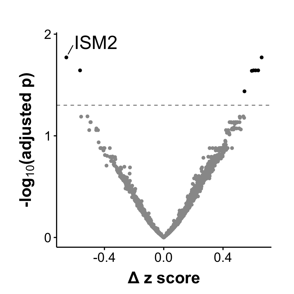
#### PE only 12wk NPXZ (logistic P)-Fig.1a
```{r ,fig.width=5,fig.height=5,volcano_purePE_12wk_npxz-function_v2, echo=FALSE, message=FALSE, fig.width=5,fig.height=5}
#POPSID+proteins+y
v1=create_volcano_plot(dataset =dl.npxz5.Roche.ISM2$PE_pure$`12wk`%>%dplyr::select(-c(Comparator, Roche_PlGF,Roche_PAPP_A,Roche_AFP,Roche_hCGbeta)),SIZE=1,"Δ z score"," ",test_type = "logistic", label_size=8,axis_number=16,axis_size=20,title_size=20,box.pad=0.1,point.pad=0.5,nudge.y=0.15,nudge.x=0.1) #npxz
print(v1)
```
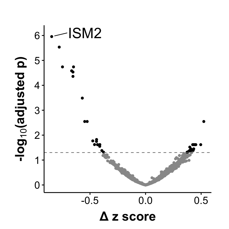
#### FGR only 12wk NPXZ (logistic P)-Fig.1b
```{r ,fig.width=5,fig.height=5,volcano_pureFGR_12wk_npxz-function_v2, echo=FALSE, message=FALSE, fig.width=5,fig.height=5}
#POPSID+proteins+y
v2=create_volcano_plot(dataset =dl.npxz5.Roche.ISM2$FGR_pure$`12wk`%>%dplyr::select(-c( Comparator,Roche_PlGF,Roche_PAPP_A,Roche_AFP,Roche_hCGbeta)),SIZE=1, "Δ z score"," ",test_type = "logistic", label_size=8,axis_number=16,axis_size=20,title_size=20,box.pad=0.1,point.pad=0.5,nudge.y=0.15,nudge.x=0.2) #npxz
print(v2)
```
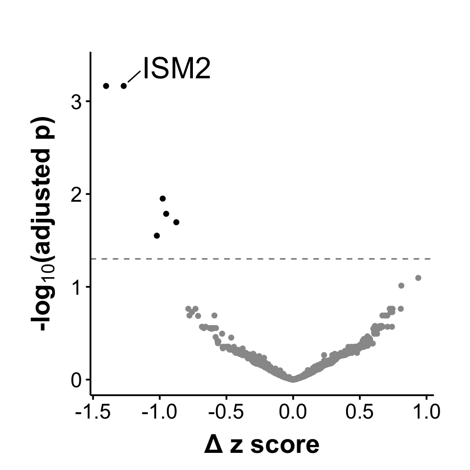
#### PE with FGR 12wk NPXZ (logistic P)-Fig.1c
```{r ,fig.width=5,fig.height=5,volcano_PE_FGR_12wk_npxz-function_v2, echo=FALSE, message=FALSE, fig.width=5,fig.height=5}
#POPSID+proteins+y
v3=create_volcano_plot(dataset =dl.npxz5.Roche.ISM2$PE_and_FGR$`12wk`%>%dplyr::select(-c( Comparator,Roche_PlGF,Roche_PAPP_A,Roche_AFP,Roche_hCGbeta,case_type)),SIZE=1,"Δ z score"," ",test_type = "logistic", label_size=8,axis_number=16,axis_size=20,title_size=20,box.pad=0.1,point.pad=0.5,nudge.y=0.2,nudge.x=0.3) #npxz
print(v3)
```
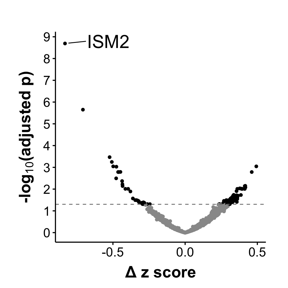
#### Composite 12wk NPXZ (logistic P)-Fig.1d
```{r ,fig.width=5,fig.height=5,volcano_Composite_12wk_npxz-function_v2, echo=FALSE, message=FALSE, fig.width=5,fig.height=5}
#POPSID+proteins+y
v4=create_volcano_plot(dataset =dl.npxz5.Roche.pops.composite.12wk%>%dplyr::select(-c( Comparator,Roche_PlGF,Roche_PAPP_A,Roche_AFP,Roche_hCGbeta))
,SIZE=1, "Δ z score"," ",test_type = "logistic", label_size=8,axis_number=16,axis_size=20,title_size=20,box.pad=0.1,point.pad=0.5,nudge.y=0.1,nudge.x=0.2) #npx
print(v4)
```
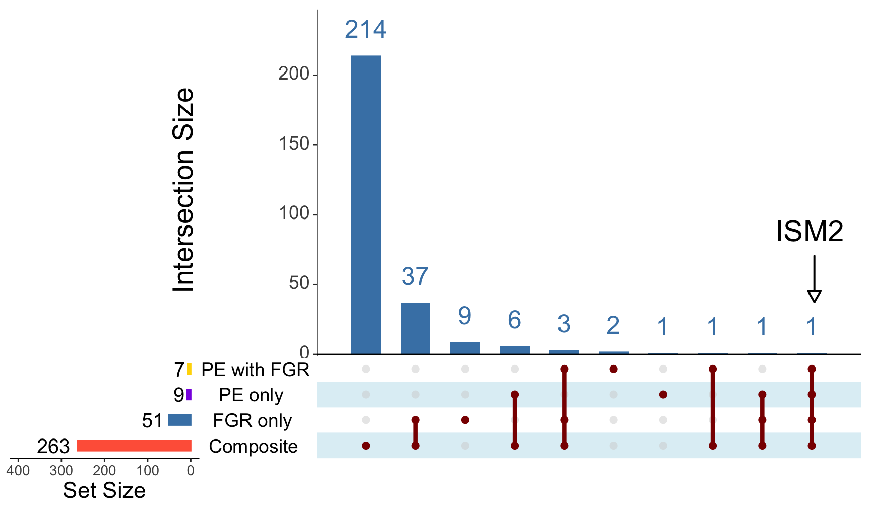
### Upset plot of DAPs-Fig.1e
```{r, fig.width=5,fig.height=5, DAPs_POPS_NPXZ_composite_upset, message=FALSE, warning=FALSE}
#POPSID+proteins+y or proteins+y
DAPs.PE=find_DEP(data.frame(dl.npxz5.Roche.ISM2$PE_pure$`12wk`%>%dplyr::select(-c(POPSID, Comparator,Roche_PlGF,Roche_PAPP_A,Roche_AFP,Roche_hCGbeta))), mc.cores = 12, pvalue = 0.05)$feature
DAPs.FGR=find_DEP(data.frame(dl.npxz5.Roche.ISM2$FGR_pure$`12wk`%>%dplyr::select(-c(POPSID, Comparator,Roche_PlGF,Roche_PAPP_A,Roche_AFP,Roche_hCGbeta))), mc.cores = 12, pvalue = 0.05)$feature
DAPs.PE.FGR=find_DEP(data.frame(dl.npxz5.Roche.ISM2$PE_and_FGR$`12wk`%>%dplyr::select(-c(POPSID, Comparator,Roche_PlGF,Roche_PAPP_A,Roche_AFP,Roche_hCGbeta,case_type))), mc.cores = 12, pvalue = 0.05)$feature
DAPs.Composite=find_DEP(data.frame(dl.npxz5.Roche.pops.composite.12wk%>%dplyr::select(-c(POPSID, Comparator,Roche_PlGF,Roche_PAPP_A,Roche_AFP,Roche_hCGbeta))), mc.cores = 12, pvalue = 0.05)$feature
#upset
all_items <- unique(c(DAPs.PE,DAPs.FGR,DAPs.PE.FGR,DAPs.Composite))
data <- data.frame(
Pure.PE = as.integer(all_items %in% DAPs.PE),
Pure.FGR = as.integer(all_items %in% DAPs.FGR),
PE.with.FGR = as.integer(all_items %in% DAPs.PE.FGR),
Composite= as.integer(all_items %in% DAPs.Composite))
rownames(data) <- all_items
names(data)[names(data) == "Pure.PE"] <- "PE only"
names(data)[names(data) == "Pure.FGR"] <- "FGR only"
names(data)[names(data) == "PE.with.FGR"] <- "PE with FGR"
```
```{r, fig.width=9, fig.height=5.3, DAPs_POPS_NPXZ_composite_upset_wider, message=FALSE, warning=FALSE}
UpSetR::upset(data,
      nsets = 4,
      nintersects = NA,
      order.by = "freq",
      decreasing = TRUE,
      mb.ratio = c(0.7, 0.3),
      number.angles = 0,
      point.size = 2.5,
      line.size = 1.5,
      main.bar.color = "steelblue",
      sets.bar.color = c("#FF6347", "#4682B4", "#8A2BE2", "#FFD700"),
      text.scale = c(2.5, 2, 2, 1.5, 2, 3),
      matrix.color = "darkred",
      shade.color = "lightblue",
      shade.alpha = 0.4,
      set_size.show = TRUE,
      set_size.numbers_size =10,
      set_size.scale_max = 400
)
grid.text("ISM2", x = 0.93, y = 0.55, gp = gpar(fontsize = 22, col = "black"))
grid.lines(x = unit(c(0.935, 0.935), "npc"),
           y = unit(c(0.5, 0.41), "npc"),
           arrow = arrow(type = "closed", length = unit(0.13, "inches")),
           gp = gpar(col = "black", lwd = 2))
```
### Logistic P value rank for top 10 proteins-Fig.1gf
Here we repeat the table of ranks but this time ranking proteins based on the P value from logistic regression rather than the AUC. We rank P from smallest to largest.
```{r fig.width=5, fig.height=5,top_P_protein, message=FALSE, warning=FALSE}
#POPSID+proteins+y or proteins+y
#pure PE
# Pure PE
P_PE_only = lreg(data.frame(dl.npxz5.Roche.ISM2$PE_pure$`12wk` %>%
dplyr::select(-c(POPSID, Comparator, Roche_PlGF, Roche_PAPP_A, Roche_AFP, Roche_hCGbeta)) %>%dplyr::rename_with(~ gsub("-", "__", .))),mc.cores = 12)
P_PE_only = P_PE_only[order(P_PE_only$pval, decreasing = F),] %>%dplyr::select(c(feature, pval)) %>%mutate(rank_p = rank(pval, ties.method = "first"))
# Pure FGR
P_FGR_only = lreg(data.frame(dl.npxz5.Roche.ISM2$FGR_pure$`12wk` %>%
 dplyr::select(-c(POPSID, Comparator, Roche_PlGF, Roche_PAPP_A, Roche_AFP, Roche_hCGbeta)) %>%dplyr::rename_with(~ gsub("-", "__", .))), mc.cores = 12)
P_FGR_only = P_FGR_only[order(P_FGR_only$pval, decreasing = F),] %>%dplyr::select(c(feature, pval)) %>%mutate(rank_p = rank(pval, ties.method = "first"))
# PE with FGR
P_PE_with_FGR = lreg(data.frame(dl.npxz5.Roche.ISM2$PE_and_FGR$`12wk` %>%
dplyr::select(-c(POPSID, Comparator, Roche_PlGF, Roche_PAPP_A, Roche_AFP, Roche_hCGbeta, case_type)) %>%dplyr::rename_with(~ gsub("-", "__", .))),mc.cores = 12)
P_PE_with_FGR = P_PE_with_FGR[order(P_PE_with_FGR$pval, decreasing = F),] %>%dplyr::select(c(feature, pval)) %>%mutate(rank_p = rank(pval, ties.method = "first"))
# composite
P_composite = lreg(data.frame(dl.npxz5.Roche.pops.composite.12wk%>%dplyr::select(-c(POPSID, Comparator,Roche_PlGF,Roche_PAPP_A,Roche_AFP,Roche_hCGbeta))%>%dplyr::rename_with(~ gsub("-", "__", .))), mc.cores=12)
P_composite = P_composite[order(P_composite$pval, decreasing = F),] %>%dplyr::select(c(feature, pval)) %>%mutate(rank_p = rank(pval, ties.method = "first"))
union_top10 = base::Reduce(base::union, list(P_PE_only$feature[1:10],P_FGR_only$feature[1:10],P_PE_with_FGR$feature[1:10],P_composite$feature[1:10]))
result_P <- data.frame(feature = union_top10,rank_p_PE_only = NA,rank_p_FGR_only = NA,rank_p_PE_with_FGR = NA,rank_p_composite = NA,p_PE_only = NA,p_FGR_onlye = NA,p_PE_with_FGR = NA,p_composite = NA)
datasets <- list(
  P_PE_only = c("p_PE_only", "rank_p_PE_only"),
  P_FGR_only = c("p_FGR_only", "rank_p_FGR_only"),
  P_PE_with_FGR = c("p_PE_with_FGR", "rank_p_PE_with_FGR"),
   P_composite = c("p_composite", "rank_p_composite"))
for (dataset_name in names(datasets)) {
  dataset <- get(dataset_name)
  p_col <- datasets[[dataset_name]][1]
  rank_p_col <- datasets[[dataset_name]][2]
  matching_rows <- dataset[dataset$feature %in% union_top10, ]
  matching_rows <- matching_rows[match(union_top10, matching_rows$feature), ]
  result_P[[p_col]] <- matching_rows$pval
  result_P[[rank_p_col]] <- matching_rows$rank_p}
result_P$rank_sum <- rowSums(result_P[, c("rank_p_PE_only", "rank_p_FGR_only", "rank_p_PE_with_FGR", "rank_p_composite")], na.rm = TRUE)
result_P$p_sum <- rowSums(result_P[, c("p_PE_only", "p_FGR_only", "p_PE_with_FGR", "p_composite")], na.rm = TRUE)
result_P <- result_P %>%
  dplyr::select(feature,
                rank_p_PE_only,
                rank_p_FGR_only,
                rank_p_PE_with_FGR,
                rank_p_composite,
                rank_sum,
                p_PE_only,
                p_FGR_only,
                p_PE_with_FGR,
                p_composite,
                p_sum) %>%
  mutate(across(c(p_PE_only, p_FGR_only, p_PE_with_FGR, p_composite,p_sum),
                ~ formatC(.x, format = "e", digits = 3))) %>%  # Convert to scientific notation
  arrange(rank_sum)
```
```{r table_rank_top_P_protein, message=FALSE, warning=FALSE}
datatable( result_P %>%
    mutate(
      across(
        c(p_PE_only, p_FGR_only, p_PE_with_FGR, p_composite, p_sum),
        ~ sprintf("%.3e", as.numeric(.))
      )
    ), rownames = FALSE, caption = "Summary of POPS serum explore",
          options = list(
            scrollX = TRUE,
            scrollCollapse = TRUE,
            order = list(4, 'asc'),
            pageLength = 40))
```
## Figure 2
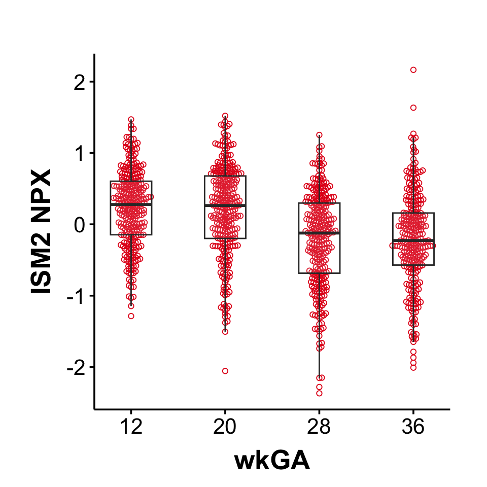
### Plot of NPX values with 4 GAs-Fig.2a
We plot NPX values vs gestational age (exact, not binned) in the control group.
```{r ,fig.width=5,fig.height=5,boxplot_NPX_POPS_ISM2, message=FALSE, warning=FALSE}
if(TRUE){
  dt.olinkID[Assay %in% dt.olinkID[,.N,Assay][N>1]$Assay]
  dt.olinkID[Assay %in% dt.olinkID[,.N,Assay][N>1]$Assay, Assay:=paste(Assay,Panel,sep=".")]
  dt.olinkID[grepl("LMOD1\\.",Assay)|grepl("SCRIB\\.",Assay)|grepl("IDO1\\.",Assay)|grepl("TNF\\.",Assay)| grepl("IL6\\.",Assay)|grepl("CXCL8\\.",Assay)]
  mat.olinkID<-dt.olinkID %>% as.matrix(rownames="OlinkID")}
dl.npx.GA <- lapply(dl.npx.GA, function(df) {
  for (l in 2:ncol(df)) {
    colnames(df)[l] <- dt.olinkID$Assay[dt.olinkID$OlinkID == colnames(df)[l]]
  }
  return(df)})
rowbind_PE=rbind(merge(phenotypes_pops_n923_anonymised %>% dplyr::select(c("Comparator","POPSID","GAwk1")), cbind(GA = 12,dl.npx.GA$`12wk`), by = "POPSID")%>%dplyr::rename(Time = GAwk1),
                 merge(phenotypes_pops_n923_anonymised %>% dplyr::select(c("Comparator","POPSID","GAwk2")), cbind(GA = 20,dl.npx.GA$`20wk`), by = "POPSID")%>%dplyr::rename(Time = GAwk2),
                 merge(phenotypes_pops_n923_anonymised %>% dplyr::select(c("Comparator","POPSID","GAwk3")), cbind(GA = 28,dl.npx.GA$`28wk`), by = "POPSID")%>%dplyr::rename(Time = GAwk3),
                 merge(phenotypes_pops_n923_anonymised %>% dplyr::select(c("Comparator","POPSID","GAwk4")), cbind(GA = 36,dl.npx.GA$`36wk`), by = "POPSID")%>%dplyr::rename(Time = GAwk4))
long_PE<- rowbind_PE[order(rowbind_PE$POPSID), ]#View(long_PE)
#Comparator+POPSID+Time+GA+proteins
################################################################POPSID+Comparator+Time+GA+proteins
long_PE<- long_PE[which(long_PE$Comparator==1), ]
b1=ggplot(long_PE, aes(x = GA, y = long_PE[,which(colnames(long_PE)=="ISM2")])) +
  geom_beeswarm(color = "#E31A1C",cex=0.9,shape = 1)+
  geom_boxplot(aes(group = GA), alpha = 0.1, outlier.shape = NA, width = 3.5) +
  labs(title = paste(" "),
       x = "wkGA", y = "ISM2 NPX") +
  scale_x_continuous(breaks = c(12, 20, 28, 36))+
  theme_Publication() +
  theme(
    panel.grid.major = element_blank(),
    panel.grid.minor = element_blank(),
    legend.title = element_blank(),
    axis.line = element_line(colour = "black"),
    axis.title = element_text(face = "bold", size = 20),
    axis.text = element_text(size = 16),
    plot.title = element_text(size = 20, face = "bold", hjust = 0.5),
    plot.margin = margin(0.5, 0.5, 0.5, 0.5, "cm")
  ) +
  coord_fixed(ratio = 1) +
  theme(
    aspect.ratio = 1
  )
print(b1)
```
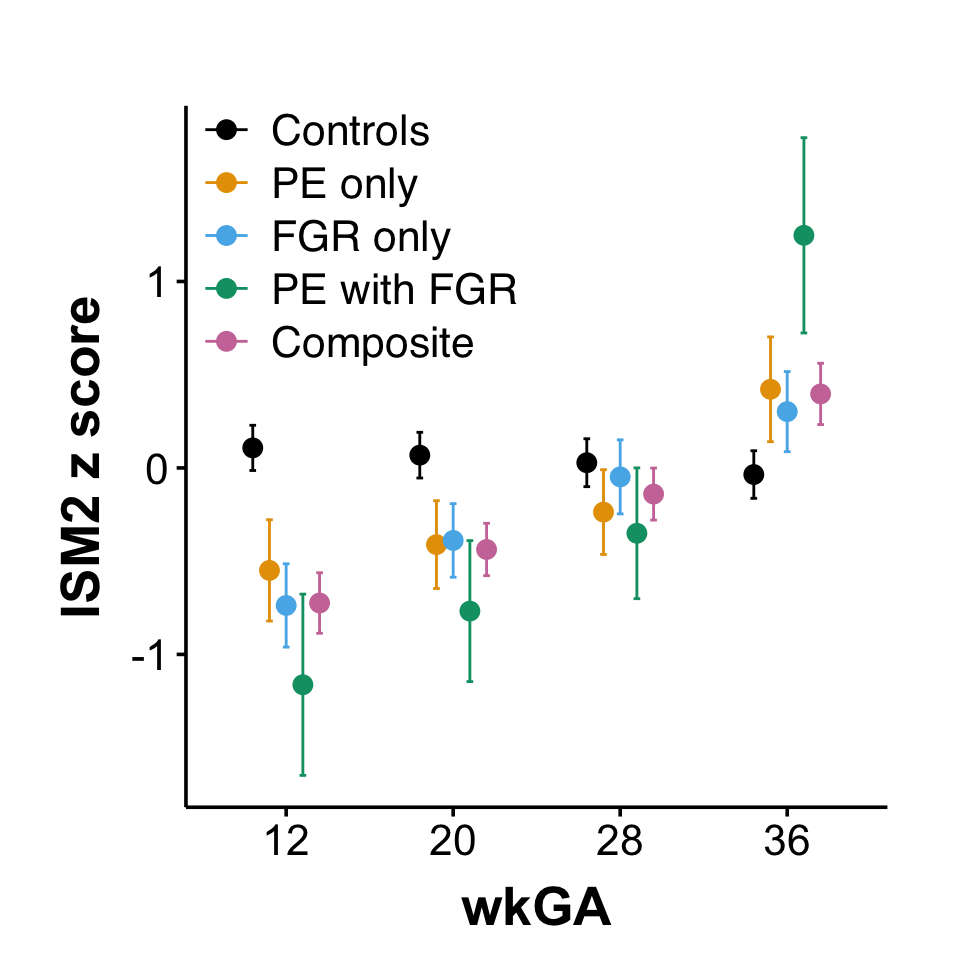
### ISM2 of the mean and 95% CI of z scores-Fig.2b
Here we have separate plot where the individual patient data has been removed and the graph simply plots the mean and 95% CI of z scores.
```{r , mean_bar_data_for_scatter_meanbar_purePE_POPS_ISM2,echo=FALSE, message=FALSE}
#data for Pure PE
PE_only_12wk=dl.npxz5.Roche.ISM2$PE_pure$`12wk`%>% dplyr::select(c("POPSID", "ISM2","y"))
PE_only_20wk=dl.npxz5.Roche.ISM2$PE_pure$`20wk`%>% dplyr::select(c("POPSID","ISM2","y"))
PE_only_28wk=dl.npxz5.Roche.ISM2$PE_pure$`28wk`%>% dplyr::select(c("POPSID","ISM2","y"))
PE_only_36wk=dl.npxz5.Roche.ISM2$PE_pure$`36wk`%>% dplyr::select(c("POPSID","ISM2","y"))
#data for Pure FGR
FGR_only_12wk=dl.npxz5.Roche.ISM2$FGR_pure$`12wk`%>% dplyr::select(c("POPSID","ISM2","y"))
FGR_only_20wk=dl.npxz5.Roche.ISM2$FGR_pure$`20wk`%>% dplyr::select(c("POPSID","ISM2","y"))
FGR_only_28wk=dl.npxz5.Roche.ISM2$FGR_pure$`28wk`%>% dplyr::select(c("POPSID","ISM2","y"))
FGR_only_36wk=dl.npxz5.Roche.ISM2$FGR_pure$`36wk`%>% dplyr::select(c("POPSID","ISM2","y"))
#data for PE and FGR
PE_FGR_12wk=dl.npxz5.Roche.ISM2$PE_and_FGR$`12wk`%>% dplyr::select(c("POPSID","ISM2","y"))
PE_FGR_20wk=dl.npxz5.Roche.ISM2$PE_and_FGR$`20wk`%>% dplyr::select(c("POPSID","ISM2","y"))
PE_FGR_28wk=dl.npxz5.Roche.ISM2$PE_and_FGR$`28wk`%>% dplyr::select(c("POPSID","ISM2","y"))
PE_FGR_36wk=dl.npxz5.Roche.ISM2$PE_and_FGR$`36wk`%>% dplyr::select(c("POPSID","ISM2","y"))
#data for composite
composite_12wk=dl.npxz5.Roche.pops.composite.12wk%>% dplyr::select(c("POPSID","ISM2","y"))
composite_20wk=dl.npxz5.Roche.pops.composite.20wk%>% dplyr::select(c("POPSID","ISM2","y"))
composite_28wk=dl.npxz5.Roche.pops.composite.28wk%>% dplyr::select(c("POPSID","ISM2","y"))
composite_36wk=dl.npxz5.Roche.pops.composite.36wk%>% dplyr::select(c("POPSID","ISM2","y"))
#merged data for controls (0,0) and both PE&FGR(1,1)
merged_12wk <- PE_only_12wk %>%
full_join(FGR_only_12wk, by = "POPSID", suffix = c("_PE", "_FGR")) %>%
full_join(PE_FGR_12wk, by = "POPSID") %>%
drop_na() %>%
dplyr::select(ISM2_PE, y_PE, y_FGR, y) %>%
dplyr::rename(ISM2 = ISM2_PE, PE = y_PE, FGR = y_FGR, PE_and_FGR = y)
merged_20wk <- PE_only_20wk %>%
full_join(FGR_only_20wk, by = "POPSID", suffix = c("_PE", "_FGR")) %>%
full_join(PE_FGR_20wk, by = "POPSID") %>%
drop_na() %>%
dplyr::select(ISM2_PE, y_PE, y_FGR, y) %>%
dplyr::rename(ISM2 = ISM2_PE, PE = y_PE, FGR = y_FGR, PE_and_FGR = y)
merged_28wk <- PE_only_28wk %>%
full_join(FGR_only_28wk, by = "POPSID", suffix = c("_PE", "_FGR")) %>%
full_join(PE_FGR_28wk, by = "POPSID") %>%
drop_na() %>%
dplyr::select(ISM2_PE, y_PE, y_FGR, y) %>%
dplyr::rename(ISM2 = ISM2_PE, PE = y_PE, FGR = y_FGR, PE_and_FGR = y)
merged_36wk <- PE_only_36wk %>%
full_join(FGR_only_36wk, by = "POPSID", suffix = c("_PE", "_FGR")) %>%
full_join(PE_FGR_36wk, by = "POPSID") %>%
drop_na() %>%
dplyr::select(ISM2_PE, y_PE, y_FGR, y) %>%
dplyr::rename(ISM2 = ISM2_PE, PE = y_PE, FGR = y_FGR, PE_and_FGR = y)
# Pure PE=1
PE_summary <- rbind(
extract_and_summarize(PE_only_12wk %>% dplyr::filter(y == 1),12, "PE only"),
extract_and_summarize(PE_only_20wk%>% dplyr::filter(y == 1), 20, "PE only"),
extract_and_summarize(PE_only_28wk%>% dplyr::filter(y == 1), 28, "PE only"),
extract_and_summarize(PE_only_36wk%>% dplyr::filter(y == 1), 36, "PE only"))
# Pure FGR=1
FGR_summary <- rbind(
extract_and_summarize(FGR_only_12wk%>% dplyr::filter(y == 1), 12, "FGR only"),
extract_and_summarize(FGR_only_20wk%>% dplyr::filter(y == 1), 20, "FGR only"),
extract_and_summarize(FGR_only_28wk%>% dplyr::filter(y == 1), 28, "FGR only"),
extract_and_summarize(FGR_only_36wk%>% dplyr::filter(y == 1), 36, "FGR only"))
# PE_and_FGR=1
PE_FGR_summary <- rbind(
extract_and_summarize(PE_FGR_12wk%>% dplyr::filter(y == 1), 12, "PE with FGR"),
extract_and_summarize(PE_FGR_20wk%>% dplyr::filter(y == 1), 20, "PE with FGR"),
extract_and_summarize(PE_FGR_28wk%>% dplyr::filter(y == 1), 28, "PE with FGR"),
extract_and_summarize(PE_FGR_36wk%>% dplyr::filter(y == 1), 36, "PE with FGR"))
# composite=1
Composite_summary <- rbind(
extract_and_summarize(composite_12wk%>% dplyr::filter(y == 1), 12, "Composite"),
extract_and_summarize(composite_20wk%>% dplyr::filter(y == 1), 20, "Composite"),
extract_and_summarize(composite_28wk%>% dplyr::filter(y == 1), 28, "Composite"),
extract_and_summarize(composite_36wk%>% dplyr::filter(y == 1), 36, "Composite"))
#common controls(0,0)
Control_summary <- bind_rows(
extract_and_summarize(merged_12wk %>% dplyr::filter(PE == 0 & FGR == 0 & PE_and_FGR == 0), 12, "Controls"),
extract_and_summarize(merged_20wk %>% dplyr::filter(PE == 0 & FGR == 0 & PE_and_FGR == 0), 20, "Controls"),
extract_and_summarize(merged_28wk %>% dplyr::filter(PE == 0 & FGR == 0 & PE_and_FGR == 0), 28, "Controls"),
extract_and_summarize(merged_36wk %>% dplyr::filter(PE == 0 & FGR == 0 & PE_and_FGR == 0), 36, "Controls"))
# Combine all summaries into one dataset
all_data <- rbind(Control_summary, PE_summary, FGR_summary,PE_FGR_summary,Composite_summary) #View(all_data)
all_data_POPS=all_data
all_data_POPS$Outcome <- factor(all_data_POPS$Outcome, levels = c("Controls", "PE only", "FGR only", "PE with FGR","Composite"))
```
```{r , auc_table_mean_bar_data_for_scatter_meanbar_purePE_POPS_ISM2,echo=FALSE, message=FALSE}
all_data$Outcome <- factor(all_data$Outcome, levels = c("Controls", "PE only", "FGR only", "PE with FGR","Composite"))
datatable(all_data , rownames = F,caption = "ISM2.12wk.as.single.measure.AUC.numbers",
options = list(
scrollX = TRUE,
scrollCollapse = TRUE,
pageLength =30)) %>%
formatRound(columns = c("Mean", "Lower_CI", "Upper_CI"), digits = 4)
scatter_data <- rbind(
PE_only_12wk%>% dplyr::filter(y == 1)%>% dplyr::select(ISM2) %>% mutate(GA = 12, Outcome = "PE only"),
PE_only_20wk%>% dplyr::filter(y == 1)%>% dplyr::select(ISM2) %>% mutate(GA = 20, Outcome= "PE only"),
PE_only_28wk%>% dplyr::filter(y == 1)%>% dplyr::select(ISM2) %>% mutate(GA = 28, Outcome= "PE only"),
PE_only_36wk%>% dplyr::filter(y == 1)%>% dplyr::select(ISM2) %>% mutate(GA = 36, Outcome= "PE only"),
FGR_only_12wk%>% dplyr::filter(y == 1)%>% dplyr::select(ISM2) %>% mutate(GA = 12, Outcome= "FGR only"),
FGR_only_20wk%>% dplyr::filter(y == 1)%>% dplyr::select(ISM2) %>% mutate(GA = 20, Outcome= "FGR only"),
FGR_only_28wk%>% dplyr::filter(y == 1)%>% dplyr::select(ISM2) %>% mutate(GA = 28, Outcome= "FGR only"),
FGR_only_36wk%>% dplyr::filter(y == 1)%>% dplyr::select(ISM2) %>% mutate(GA = 36, Outcome= "FGR only"),
PE_FGR_12wk%>% dplyr::filter(y == 1)%>% dplyr::select(ISM2)%>% mutate(GA = 12, Outcome= "PE with FGR"),
PE_FGR_20wk%>% dplyr::filter(y == 1)%>% dplyr::select(ISM2)%>% mutate(GA = 20, Outcome= "PE with FGR"),
PE_FGR_28wk%>% dplyr::filter(y == 1)%>% dplyr::select(ISM2)%>% mutate(GA = 28, Outcome= "PE with FGR"),
PE_FGR_36wk%>% dplyr::filter(y == 1)%>% dplyr::select(ISM2)%>% mutate(GA = 36, Outcome= "PE with FGR"),
composite_12wk%>% dplyr::filter(y == 1)%>% dplyr::select(ISM2)%>% mutate(GA = 12,Outcome= "Composite"),
composite_20wk%>% dplyr::filter(y == 1)%>% dplyr::select(ISM2)%>% mutate(GA = 20, Outcome= "Composite"),
composite_28wk%>% dplyr::filter(y == 1)%>% dplyr::select(ISM2)%>% mutate(GA = 28, Outcome= "Composite"),
composite_36wk%>% dplyr::filter(y == 1)%>% dplyr::select(ISM2)%>% mutate(GA = 36, Outcome= "Composite"),
merged_12wk %>% dplyr::filter(PE == 0 & FGR == 0 & PE_and_FGR == 0)%>% dplyr::select(ISM2) %>% mutate(GA = 12, Outcome= "Controls"),
merged_20wk %>% dplyr::filter(PE == 0 & FGR == 0 & PE_and_FGR == 0)%>% dplyr::select(ISM2) %>% mutate(GA = 20, Outcome= "Controls"),
merged_28wk %>% dplyr::filter(PE == 0 & FGR == 0 & PE_and_FGR == 0)%>% dplyr::select(ISM2) %>% mutate(GA = 28, Outcome= "Controls"),
merged_36wk %>% dplyr::filter(PE == 0 & FGR == 0 & PE_and_FGR == 0)%>% dplyr::select(ISM2) %>% mutate(GA = 36, Outcome= "Controls"))
scatter_data_POPS=scatter_data
scatter_data_POPS$Outcome <- factor(scatter_data_POPS$Outcome, levels = c("Controls", "PE only", "FGR only", "PE with FGR","Composite"))
```
```{r ,fig.width=5,fig.height=5,scatter_meanbar_purePE_POPS_ISM2,echo=FALSE, message=FALSE}
######################################################################
m1=ggplot() +
geom_errorbar(data = all_data, aes(x = factor(GA), y = Mean,
ymin = Lower_CI, ymax = Upper_CI, color = Outcome),
width = 0.2, position = position_dodge(0.5)) +
geom_point(data = all_data, aes(x = factor(GA), y = Mean, color = Outcome, fill = Outcome),
position = position_dodge(0.5), size = 3, shape = 21) +
labs(
title = " ",
x = "wkGA",
y = "ISM2 z score",
fill = "Outcome",
color = "Outcome") +
scale_color_manual(values = c("Controls" = "#000000",
"PE only" = "#E69F00",
"FGR only" = "#56B4E9",
"PE with FGR" = "#009E73",
"Composite" = "#CC79A7")) +
scale_fill_manual(values = c("Controls" = "#000000",
"PE only" = "#E69F00",
"FGR only" = "#56B4E9",
"PE with FGR" = "#009E73",
"Composite" = "#CC79A7")) +
scale_x_discrete(labels = c("12", "20", "28", "36")) +
scale_y_continuous(labels = function(x) round(x, 2)) +
theme_Publication() +
theme(legend.position = c(0.5, 0.6),
legend.justification = c("right", "bottom"),
legend.background = element_rect(fill = alpha("white", 0)),
legend.key = element_blank(),
panel.grid.major = element_blank(),
panel.grid.minor = element_blank(),
legend.title = element_blank(),
legend.text = element_text(size = 16),
axis.line = element_line(colour = "black"),
axis.title = element_text(face = "bold", size = 20),
axis.text = element_text(size = 16),
plot.title = element_text(size = 20, face = "bold", hjust = 0.5),
plot.margin = margin(0.5, 0.5, 0.5, 0.5, "cm"),
aspect.ratio = 1 ) +
coord_fixed(ratio = 1)
print(m1)
```
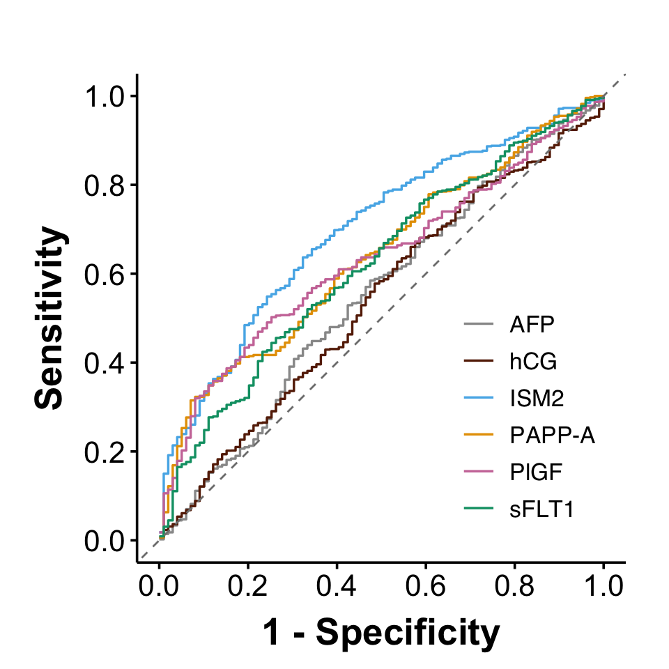
### ROC curves of ISM2 from composite of all three outcomes with the five Roche biomarkers in POPS-Fig.2c
ROC curves for ISM2 with the five Roche biomarkers (PAPP-A, sFLT1, PlGF, hCG and AFP)
```{r Logistic_POPS_ISM2-biomarkers-composite, message=FALSE, warning=FALSE}
#Composite
df_POPS_composite <-dl.npxz5.Roche.pops.composite.12wk%>%
  dplyr::select(c("ISM2","y"))
df_POPS_composite_Roche_sFLT1 <- dl.npxz5.Roche.pops.composite.12wk%>%
  dplyr::select(c("Roche_sFLT1","y"))
df_POPS_composite_PlGF <- dl.npxz5.Roche.pops.composite.12wk%>%
  dplyr::select(c("Roche_PlGF","y"))
df_POPS_composite_Roche_PAPP_A <- dl.npxz5.Roche.pops.composite.12wk%>%
  dplyr::select(c("Roche_PAPP_A","y"))
df_POPS_composite_Roche_AFP <-dl.npxz5.Roche.pops.composite.12wk%>%
  dplyr::select(c("Roche_AFP","y"))
df_POPS_composite_Roche_hCGbeta <- dl.npxz5.Roche.pops.composite.12wk%>%
  dplyr::select(c("Roche_hCGbeta","y"))
results <- rbind(
  cbind(Cohort = "POPS composite 12wk", lreg(df_POPS_composite, mc.cores=12)),
  cbind(Cohort = "POPS composite 12wk", lreg(df_POPS_composite_Roche_sFLT1, mc.cores=12)),
  cbind(Cohort = "POPS composite 12wk", lreg(df_POPS_composite_PlGF, mc.cores=12)),
  cbind(Cohort = "POPS composite 12wk", lreg(df_POPS_composite_Roche_PAPP_A, mc.cores=12)),
  cbind(Cohort = "POPS composite 12wk", lreg(df_POPS_composite_Roche_AFP, mc.cores=12)),
  cbind(Cohort = "POPS composite 12wk", lreg(df_POPS_composite_Roche_hCGbeta, mc.cores=12)))
results <- results %>%
  mutate(pval = formatC(pval, format = "e", digits = 3))%>%
  mutate(across(where(is.numeric), ~ round(.x, 4)))
datatable(results, rownames = F,caption = "AUC for ISM2 from composite of all three outcomes with the five Roche biomarkers",
          options = list(
            scrollX = TRUE,
            scrollCollapse = TRUE,
            pageLength =30))
```
```{r ,fig.width=5,fig.height=5,ISM2_ROC_biomarkers-composite, message=FALSE, warning=FALSE}
PE_data_train <- dl.npxz5.Roche.pops.composite.12wk
compute_roc <- function(biomarker, data) {
  model <- glm(y ~ ., data = data %>% dplyr::select(c(biomarker, "y")), family = binomial)
  log_likelihood_full <- logLik(model)
  log_likelihood_null <- logLik(glm(y ~ 1, data = data, family = binomial))
  modelLR <- -2 * (log_likelihood_null - log_likelihood_full)
  df <- length(coef(model)) - 1
  s <- as.numeric((modelLR - df) / modelLR)
  coefficients_original <- coef(model)[-1]
  coefficients_shrunk <- s * coefficients_original
  intercept <- coef(model)[1]
  data$linpred <- intercept + rowSums(
    sapply(names(coefficients_shrunk), function(protein) {
      data[[protein]] * coefficients_shrunk[protein]}))
  data$predrisk <- 1 / (1 + exp(-data$linpred))
  roc_curve <- roc(data$y, data$predrisk)
  return(roc_curve)}
# Compute ROC curves for ISM2 and each Roche biomarker
roc_ism2 <- compute_roc("ISM2", PE_data_train)
roc_pappa <- compute_roc("Roche_PAPP_A", PE_data_train)
roc_sflt1 <- compute_roc("Roche_sFLT1", PE_data_train)
roc_plgf  <- compute_roc("Roche_PlGF", PE_data_train)
roc_hcg   <- compute_roc("Roche_hCGbeta", PE_data_train)
roc_afp   <- compute_roc("Roche_AFP", PE_data_train)
auc_values <- c(ISM2  = auc(roc_ism2),PAPPA = auc(roc_pappa),sFLT1 = auc(roc_sflt1),PlGF  = auc(roc_plgf),hCG   = auc(roc_hcg),AFP   = auc(roc_afp))
auc_sorted <- sort(auc_values, decreasing = TRUE)
# Perform DeLong's test: ISM2 vs each biomarker
p_pappa <- roc.test(roc_ism2, roc_pappa, method = "delong")$p.value
p_sflt1 <- roc.test(roc_ism2, roc_sflt1, method = "delong")$p.value
p_plgf  <- roc.test(roc_ism2, roc_plgf, method = "delong")$p.value
p_hcg   <- roc.test(roc_ism2, roc_hcg, method = "delong")$p.value
p_afp   <- roc.test(roc_ism2, roc_afp, method = "delong")$p.value
cat("P-values comparing ISM2 to other biomarkers:\n")
cat("PAPP-A vs ISM2: ", p_pappa, "\n")
cat("sFLT1 vs ISM2:", p_sflt1, "\n")
cat("PlGF vs ISM2: ", p_plgf, "\n")
cat("hCG vs ISM2: ", p_hcg, "\n")
cat("AFP vs ISM2: ", p_afp, "\n")
```
```{r ,fig.width=5,fig.height=5,ISM2_ROC_POPS_biomarkers-composite_nolegend, message=FALSE, warning=FALSE}
interpolate_roc <- function(roc_obj, n = 100) {
  specificity <- roc_obj$specificities
  sensitivity <- roc_obj$sensitivities
  new_specificity <- seq(0, 1, length.out = n)
  new_sensitivity <- approx(specificity, sensitivity, xout = new_specificity)$y
  return(data.frame(Specificity = new_specificity, Sensitivity = new_sensitivity))}
roc_ism2_interp <- interpolate_roc(roc_ism2)
roc_pappa_interp <- interpolate_roc(roc_pappa)
roc_plgf_interp <- interpolate_roc(roc_plgf)
roc_sflt1_interp <- interpolate_roc(roc_sflt1)
roc_hcg_interp <- interpolate_roc(roc_hcg)
roc_afp_interp <- interpolate_roc(roc_afp)
roc_df <- rbind(
  cbind(roc_ism2_interp, Group = "ISM2"),
  cbind(roc_pappa_interp, Group = "PAPP-A"),
  cbind(roc_plgf_interp, Group = "PlGF"),
  cbind(roc_sflt1_interp, Group = "sFLT1"),
  cbind(roc_hcg_interp, Group = "hCG"),
  cbind(roc_afp_interp, Group = "AFP"))
auc_values <- c(auc(roc_ism2), auc(roc_pappa), auc(roc_plgf), auc(roc_sflt1), auc(roc_hcg), auc(roc_afp))
p_values <- c(p_pappa, p_sflt1, p_plgf, p_hcg, p_afp)
r5 <- ggplot(roc_df, aes(x = 1 - Specificity, y = Sensitivity,
                         color = Group, linetype = Group)) +
  geom_step(size = 0.6, direction = "hv") +
  geom_abline(slope = 1, intercept = 0,
              linetype = "dashed", color = "gray50") +
  labs(
    title = "",
    x = "1 - Specificity",
    y = "Sensitivity"
  ) +
  scale_x_continuous(limits = c(0, 1), breaks = seq(0, 1, 0.2)) +
  scale_y_continuous(limits = c(0, 1), breaks = seq(0, 1, 0.2)) +
  scale_color_manual(values = c(
    "ISM2" = "#56B4E9",
    "PAPP-A" = "#E69F00",
    "PlGF" = "#CC79A7",
    "sFLT1" = "#009E73",
    "AFP" = "#999999",
    "hCG" = "#662506"
  )) +
  scale_linetype_manual(values = rep("solid", 6)) +
  theme_Publication() +
  theme(
    legend.position = c(0.8, 0.3),
    panel.grid.major = element_blank(),
    panel.grid.minor = element_blank(),
    legend.title = element_blank(),
    axis.line = element_line(colour = "black"),
    axis.title = element_text(face = "bold", size = 20),
    axis.text = element_text(size = 16),
    plot.title = element_text(size = 20, face = "bold", hjust = 0.5),
    plot.margin = margin(0.5, 0.5, 0.5, 0.5, "cm"),
    aspect.ratio = 1
  ) +
  coord_fixed(ratio = 1)
print(r5)
```
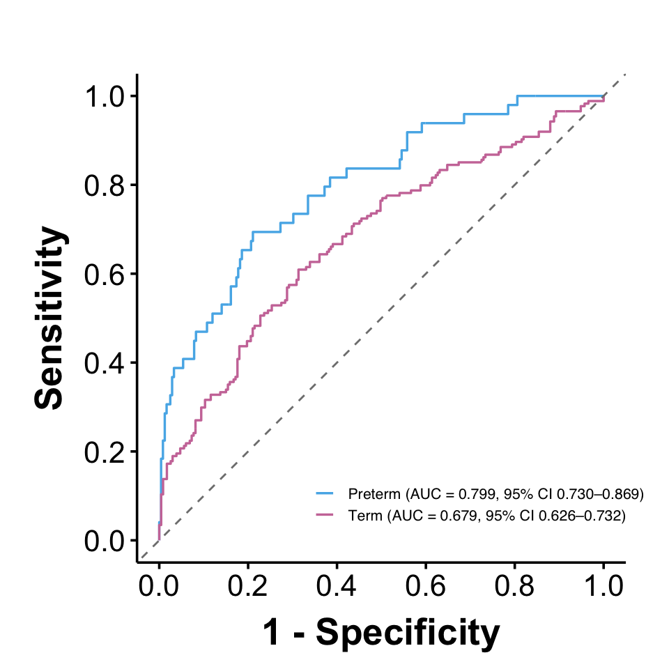
### AUCs for POPS in composite outcome (controls vs. cases) restricted to cases resulting in preterm birth versus term birth at 12wkGA-Fig.2d
```{r,fig.width=5,fig.height=5,AUC_pre_term_ISM2_composite, message=FALSE, warning=FALSE}
plot_roc_preterm_term <- function(data_preterm, data_term, protein_col, outcome_col, title) {
  condition_colors <- c(
    "Preterm" = "#56B4E9",
    "Term"    = "#CC79A7"
  )
  get_roc_df <- function(data, label_name) {
    df <- data %>%
      dplyr::select(all_of(c(protein_col, outcome_col))) %>%
      dplyr::rename(y = all_of(outcome_col)) %>%
      tidyr::drop_na()
    # Fit model
    fit <- glm(y ~ ., data = df, family = binomial)
    # Shrinkage
    ll_full <- logLik(fit)
    ll_null <- logLik(glm(y ~ 1, data = df, family = binomial))
    modelLR <- -2 * (ll_null - ll_full)
    df_model <- length(coef(fit)) - 1
    s <- as.numeric((modelLR - df_model) / modelLR)
    coefs <- coef(fit)
    intercept <- coefs[1]
    beta <- s * coefs[-1]
    # Linear predictor
    linpred <- intercept + as.matrix(df[, protein_col]) %*% beta
    df$pred <- 1 / (1 + exp(-linpred))
    # ROC
    roc_obj <- pROC::roc(df$y, df$pred, quiet = TRUE)
    # AUC + CI
    auc_val <- pROC::auc(roc_obj)
    ci <- pROC::ci.auc(roc_obj, conf.level = 0.95)
    # Legend label WITH CI
    label <- sprintf(
      "%s (AUC = %.3f, 95%% CI %.3f–%.3f)",
      label_name,
      auc_val,
      ci[1],
      ci[3]    )
    data.frame(
      Specificity = roc_obj$specificities,
      Sensitivity = roc_obj$sensitivities,
      Group = label_name,
      Label = label   )  }
  roc_df <- rbind(
    get_roc_df(data_preterm, "Preterm"),
    get_roc_df(data_term, "Term")
  ) %>%
    dplyr::distinct(Group, Specificity, Sensitivity, .keep_all = TRUE) %>%
    dplyr::arrange(Group, Specificity, Sensitivity)
  p <- ggplot(roc_df, aes(
    x = 1 - Specificity,
    y = Sensitivity,
    color = Group,
    linetype = Group
  )) +
    geom_step(size = 0.6, direction = "hv") +
    geom_abline(slope = 1, intercept = 0,
                linetype = "dashed", color = "gray50") +
    labs(
      title = title,
      x = "1 - Specificity",
      y = "Sensitivity"
    ) +
    scale_x_continuous(limits = c(0, 1), breaks = seq(0, 1, 0.2)) +
    scale_y_continuous(limits = c(0, 1), breaks = seq(0, 1, 0.2)) +
    scale_color_manual(values = condition_colors,
                       labels = unique(roc_df$Label)) +
    scale_linetype_manual(values = c("Preterm" = "solid", "Term" = "solid"),
                          labels = unique(roc_df$Label)) +
    theme_Publication() +
    theme(
      legend.position = c(0.7, 0.12),
      legend.title = element_blank(),
      legend.text = element_text(size = 8),
      legend.key.size = unit(0.8, "lines"),
      panel.grid.major = element_blank(),
      panel.grid.minor = element_blank(),
      axis.line = element_line(colour = "black"),
      axis.title = element_text(face = "bold", size = 20),
      axis.text = element_text(size = 16),
      plot.title = element_text(size = 20, face = "bold", hjust = 0.5),
      plot.margin = margin(0.5, 0.5, 0.5, 0.5, "cm"),
      aspect.ratio = 1
    ) +
    coord_fixed(ratio = 1)
  return(list(
    plot = p,
    roc_data = roc_df
  ))
}
res <- plot_roc_preterm_term(
  data_preterm = dl.npxz5.Roche.final$PE_FGR_com_pt$`12wk`,
  data_term    = dl.npxz5.Roche.final$PE_FGR_com_t$`12wk`,
  protein_col  = "ISM2",
  outcome_col  = "y",
  title = " "
)
print(res$plot)
```
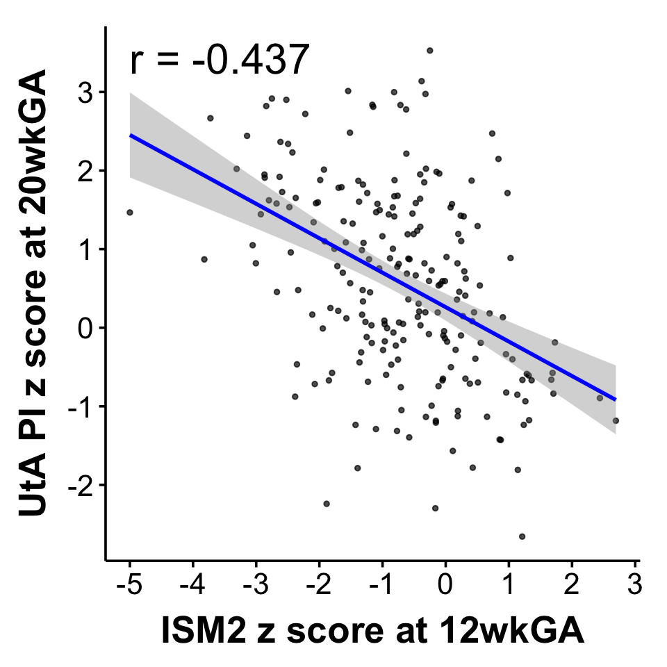
### UtA mean PI vs ISM2-Fig.2e: Cases only
```{r,fig.width=5,fig.height=5,Fig_2e_Scatter_an_scan2_logutmpiZv2_ISM2_cases, message=FALSE, warning=FALSE}
data=UtA_PI_Age_BMI_Roche_pops_12wk_com
case_data <- data %>%
  dplyr::filter(PE_FGR_com == 1, !is.na(ISM2), !is.na(an_scan2_logutmpiZv2))
cor_test_case <- cor.test(case_data$ISM2, case_data$an_scan2_logutmpiZv2)
print(cor_test_case)
correlation_coefficient <- stats::cor(case_data$ISM2, case_data$an_scan2_logutmpiZv2)
model_case <- lm(an_scan2_logutmpiZv2 ~ ISM2, data = case_data)
summary(model_case)
fig_2e <- ggplot(case_data, aes(x = ISM2, y = an_scan2_logutmpiZv2)) +
  geom_point(size = 1, alpha = 0.7) +
  geom_smooth(method = "lm", se = TRUE, color = "blue") +
  labs(
    x = "ISM2 z score at 12wkGA",
    y = "UtA PI z score at 20wkGA" ) +
  annotate("text", x = min(case_data$ISM2), y = max(case_data$an_scan2_logutmpiZv2) - 0.1,
           label = paste0("r = ", round(correlation_coefficient, 3)),
           hjust = 0, size = 8, color = "black") +
  scale_x_continuous(breaks = seq(-5, 3, 1)) +
  scale_y_continuous(breaks = seq(-3, 4, 1)) +
  theme_Publication() +
  theme(legend.position = "none",
        panel.grid.major = element_blank(),
        panel.grid.minor = element_blank(),
        legend.title = element_blank(),
        axis.line = element_line(colour = "black"),
        axis.title = element_text(face = "bold", size = 20),
        axis.text = element_text(size = 16),
        plot.title = element_text(size = 20, face = "bold", hjust = 0.5),
        plot.margin = margin(0.5, 0.5, 0.5, 0.5, "cm"),
        aspect.ratio = 1
  ) +coord_fixed(ratio = 1)
print(fig_2e)
```
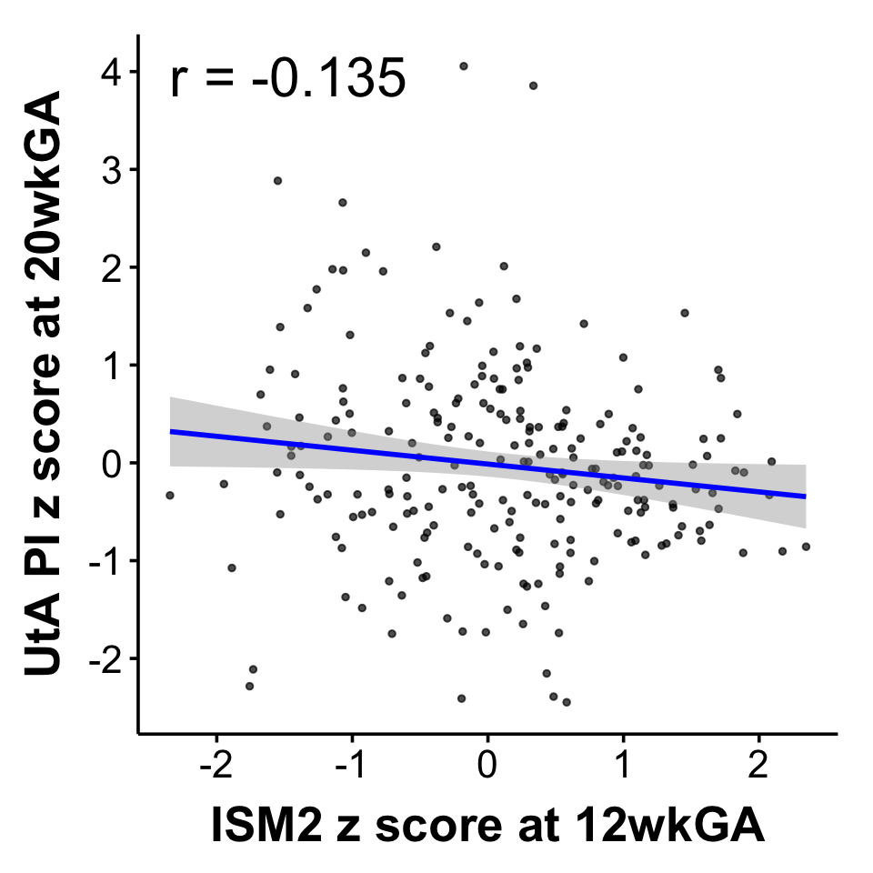
### UtA mean PI vs ISM2-Fig.2f:Controls only
```{r,fig.width=5,fig.height=5,Fig_2f_Scatter_an_scan2_logutmpiZv2_ISM2_controls, message=FALSE, warning=FALSE}
control_data <- data %>%dplyr::filter(PE_FGR_com == 0, !is.na(ISM2), !is.na(an_scan2_logutmpiZv2))
cor_test_ctrl <- cor.test(control_data$ISM2, control_data$an_scan2_logutmpiZv2)
print(cor_test_ctrl)
correlation_coefficient <- stats::cor(control_data$ISM2, control_data$an_scan2_logutmpiZv2)
model_ctrl <- lm(an_scan2_logutmpiZv2 ~ ISM2, data = control_data)
summary(model_ctrl)
fig_2f <- ggplot(control_data, aes(x = ISM2, y = an_scan2_logutmpiZv2)) +
  geom_point(size = 1, alpha = 0.7) +
  geom_smooth(method = "lm", se = TRUE, color = "blue") +
  labs(
    x = "ISM2 z score at 12wkGA",
    y = "UtA PI z score at 20wkGA" ) +annotate("text", x = min(control_data$ISM2), y = max(control_data$an_scan2_logutmpiZv2) - 0.1,
    label = paste0("r = ", round(correlation_coefficient, 3)),
    hjust = 0, size = 8, color = "black") +
  scale_x_continuous(breaks = seq(-3, 3, 1)) +
  scale_y_continuous(breaks = seq(-3, 4, 1)) +
  theme_Publication() +
  theme(legend.position = "none",
        panel.grid.major = element_blank(),
        panel.grid.minor = element_blank(),
        legend.title = element_blank(),
        axis.line = element_line(colour = "black"),
        axis.title = element_text(face = "bold", size = 20),
        axis.text = element_text(size = 16),
        plot.title = element_text(size = 20, face = "bold", hjust = 0.5),
        plot.margin = margin(0.5, 0.5, 0.5, 0.5, "cm"),
        aspect.ratio = 1
  ) +coord_fixed(ratio = 1)
print(fig_2f)
```
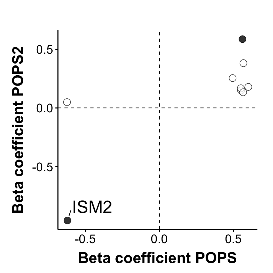
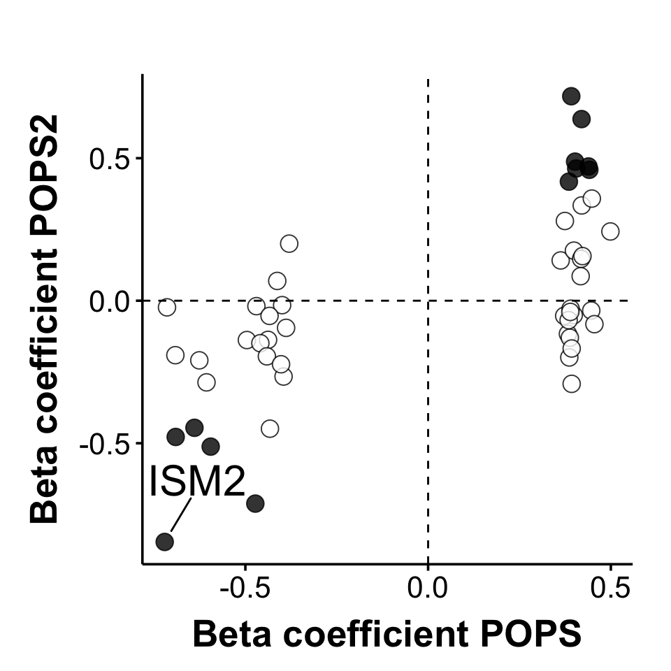
### Scatters of logistic regression beta coefficients for PE only 12wk-Fig.2g
In the X/Y plot, please only include points which were DAPs in POPS. Do not include the proteins which were not DAPs. In that plot, please colour the symbol according to the unadjusted P value for the given protein in the POPS2 validation.
```{r,fig.width=5,fig.height=5,validation_POPS2_DAPs_prurePE_12wk-DAPs_line, message=FALSE, warning=FALSE}
#proteins+Y
#########logistic: coefficients
#POPSID+proteins+y or proteins+y
### POPS
log_X=lreg(data.frame(dl.npxz5.Roche.ISM2$PE_pure$`12wk`%>%dplyr::select(-c(POPSID, Comparator,Roche_PlGF,Roche_PAPP_A,Roche_AFP,Roche_hCGbeta))%>%dplyr::rename(y = last_col())), mc.cores=12)
### validation
log_Y=lreg(data.frame(dl.npxz5.pops2.ISM2$`12wk`$PE_pure%>%dplyr::select(-c(POPSID))%>%dplyr::rename(y = last_col())),mc.cores=12)
##################
#FDR for DAPs
#POPSID+proteins+y or proteins+y
DAPs_X<- find_DEP(data.frame(dl.npxz5.Roche.ISM2$PE_pure$`12wk`%>%dplyr::select(-c(POPSID, Comparator,Roche_PlGF,Roche_PAPP_A,Roche_AFP,Roche_hCGbeta))%>%dplyr::rename(y = last_col())),  mc.cores=12,pvalue=0.05)
DAPs_Y<- find_DEP(data.frame(dl.npxz5.pops2.ISM2$`12wk`$PE_pure%>%dplyr::select(-c(POPSID))%>%dplyr::rename(y = last_col())),  mc.cores=12,pvalue=0.05)
############################scatter with label and groups
merged_data <- inner_join(
  log_X %>%dplyr::select(feature, log_odds) %>% dplyr::rename(x = log_odds),
  log_Y %>% dplyr::select(feature, log_odds,pval) %>% dplyr::rename(y = log_odds),
  by = "feature")
data <- data.frame(
  features=merged_data$feature,
  x = merged_data$x,
  y = merged_data$y,
  color=merged_data$pval,
  re_color=log10(merged_data$pval)
)
##########################################discordant & concordant
#################proteins and DEPs in each quadrant
data$quadrant=ifelse(data$x>0 & data$y>0, 1,
                     ifelse(data$x>0  & data$y<0, 4,
                            ifelse(data$x<0  & data$y>0, 2, 3  )   ))
#########color DEPs and non DEPs
overlap=base::intersect(DAPs_X$feature,DAPs_Y$feature)
x_only=base::setdiff(DAPs_X$feature, DAPs_Y$feature)
y_only=base::setdiff(DAPs_Y$feature,DAPs_X$feature)
data$label <- ifelse(data$features %in% overlap, "overlap",
                     ifelse(data$features %in% x_only, "POPS_DAPs_only",
                            ifelse(data$features %in% y_only, "POPS2_DAPs_only", "non_DAPs")))
#########################################################################discordant & concordant
#extract proteins for DAPs from POPS
data= data %>%dplyr::filter(features %in% DAPs_X$feature) #View(data)
######################################################################
######################################################################
#Restore - in Specific Protein Names
# Replace "." with "-" for specific proteins
data$features<- gsub("^NT\\.proBNP$", "NT-proBNP", data$features)
data$features <- gsub("^HLA\\.DRA$", "HLA-DRA", data$features)
data$features<- gsub("^HLA\\.E$", "HLA-E",data$features)
data$features<- gsub("^ERVV\\.1$", "ERVV-1",data$features)
data$features<- gsub("^HLA\\.A$", "HLA-A", data$features)
######################################################################
######################################################################
correlation_coefficient <- stats::cor(data$x, data$y, method = "spearman")
lm_model <- lm(y ~ x, data = data)
######################################################################
######################################################################
data$P_value <- ifelse(data$color < 0.05, "black", "white")
s1=ggplot(data, aes(x = x, y = y)) +
  geom_point(aes(fill = P_value), shape = 21, size = 4, stroke = 0.5, alpha = 0.8) +
  xlab("Beta coefficient POPS") +
  ylab("Beta coefficient POPS2") +
  ggtitle("") +
  geom_hline(yintercept = 0, linetype = "dashed", color = "black") +
  geom_vline(xintercept = 0, linetype = "dashed", color = "black") +
  theme(panel.background = element_rect(fill = "white")) +
  scale_fill_manual(values = c("black", "white"), labels = c("P < 0.05", "P ≥ 0.05")) +
  guides(fill = guide_legend(title = NULL)) +  # Hide legend title
  geom_text_repel(data = subset(data, features == "ISM2"), aes(label = features),
                  hjust = 0.8, vjust = 0.8, size = 8, color = "black",
                  nudge_y = 0.15, nudge_x = 0.25,
                  box.padding=0.2,point.padding=0.8,
                  segment.size = 0.5,segment.curvature = 0, direction = "y" ) +
   scale_x_continuous(breaks = c(-0.5, 0, 0.5, 1)) +
  scale_y_continuous(breaks = c(-0.5, 0, 0.5, 1)) +
  theme_Publication() +
    theme( legend.position = "none",
     panel.grid.major = element_blank(),
    panel.grid.minor = element_blank(),
    legend.title = element_blank(),
    axis.line = element_line(colour = "black"),
    axis.title = element_text(face = "bold", size = 20),
    axis.text = element_text(size = 16),
    plot.title = element_text(size = 20, face = "bold", hjust = 0.5),
    plot.margin = margin(0.5, 0.5, 0.5, 0.5, "cm"),
    ) +
  coord_fixed(ratio = 1) +
  theme(
    aspect.ratio = 1
  )
print(s1)
```
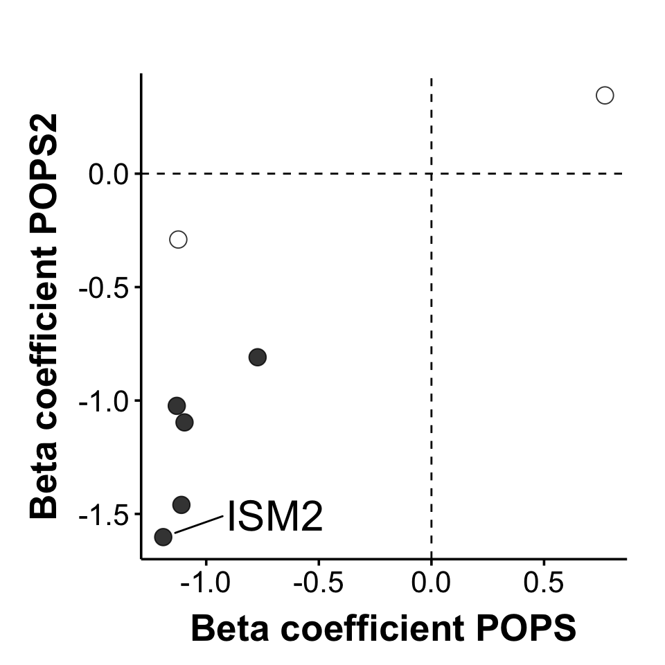
### Scatters of logistic regression beta coefficients for FGR only 12wk-Fig.2h
```{r ,fig.width=5,fig.height=5,validation_POPS2_DAPs_prureFGR_12wk-DAPs_line, message=FALSE, warning=FALSE}
log_X=lreg(data.frame(dl.npxz5.Roche.ISM2$FGR_pure$`12wk`%>%dplyr::select(-c(POPSID, Comparator,Roche_PlGF,Roche_PAPP_A,Roche_AFP,Roche_hCGbeta))%>%dplyr::rename(y = last_col())), mc.cores=12)
log_Y=lreg(data.frame(dl.npxz5.pops2.ISM2$`12wk`$FGR_pure%>%dplyr::select(-c(POPSID))%>%dplyr::rename(y = last_col())),mc.cores=12)
DAPs_X<- find_DEP(data.frame(dl.npxz5.Roche.ISM2$FGR_pure$`12wk`%>%dplyr::select(-c(POPSID, Comparator,Roche_PlGF,Roche_PAPP_A,Roche_AFP,Roche_hCGbeta))%>%dplyr::rename(y = last_col())),  mc.cores=12,pvalue=0.05)
DAPs_Y<- find_DEP(data.frame(dl.npxz5.pops2.ISM2$`12wk`$FGR_pure%>%dplyr::select(-c(POPSID))%>%dplyr::rename(y = last_col())),  mc.cores=12,pvalue=0.05)
merged_data <- inner_join(
  log_X %>%dplyr::select(feature, log_odds) %>% dplyr::rename(x = log_odds),
  log_Y %>% dplyr::select(feature, log_odds,pval) %>% dplyr::rename(y = log_odds),
  by = "feature")
data <- data.frame(
  features=merged_data$feature,
  x = merged_data$x, #POPS
  y = merged_data$y,  #validation
  color=merged_data$pval,
  re_color=log10(merged_data$pval) )
data$quadrant=ifelse(data$x>0 & data$y>0, 1,
                     ifelse(data$x>0  & data$y<0, 4,
                            ifelse(data$x<0  & data$y>0, 2, 3  )   ))
overlap=base::intersect(DAPs_X$feature,DAPs_Y$feature)
x_only=base::setdiff(DAPs_X$feature, DAPs_Y$feature)
y_only=base::setdiff(DAPs_Y$feature,DAPs_X$feature)
data$label <- ifelse(data$features %in% overlap, "overlap",
                     ifelse(data$features %in% x_only, "POPS_DAPs_only",
                            ifelse(data$features %in% y_only, "POPS2_DAPs_only", "non_DAPs")))
data= data %>%dplyr::filter(features %in% DAPs_X$feature)
data$features<- gsub("^NT\\.proBNP$", "NT-proBNP", data$features)
data$features <- gsub("^HLA\\.DRA$", "HLA-DRA", data$features)
data$features<- gsub("^HLA\\.E$", "HLA-E",data$features)
data$features<- gsub("^ERVV\\.1$", "ERVV-1",data$features)
data$features<- gsub("^HLA\\.A$", "HLA-A", data$features)
correlation_coefficient <- stats::cor(data$x, data$y, method = "spearman")
lm_model <- lm(y ~ x, data = data)
data$P_value <- ifelse(data$color < 0.05, "black", "white")
s2=ggplot(data, aes(x = x, y = y)) +
  geom_point(aes(fill = P_value), shape = 21, size = 4, stroke = 0.5, alpha = 0.8) +
  xlab("Beta coefficient POPS") +
  ylab("Beta coefficient POPS2") +
  ggtitle("") +
  geom_hline(yintercept = 0, linetype = "dashed", color = "black") +
  geom_vline(xintercept = 0, linetype = "dashed", color = "black") +
  theme(panel.background = element_rect(fill = "white")) +
  scale_fill_manual(values = c("black", "white"), labels = c("P < 0.05", "P ≥ 0.05")) +
  guides(fill = guide_legend(title = NULL)) +
  geom_text_repel(data = subset(data, features == "ISM2"), aes(label = features),
                  hjust = 0.8, vjust = 0.8, size = 8, color = "black",
                  nudge_y = 0.25, nudge_x = 0.15,
                  box.padding=0.2,point.padding=0.8,
                  segment.size = 0.5,segment.curvature = 0, direction = "y" ) +
   scale_x_continuous(breaks = c(-0.5, 0, 0.5, 1)) +
  scale_y_continuous(breaks = c(-0.5, 0, 0.5, 1)) +
  theme_Publication() +
    theme( legend.position = "none",
     panel.grid.major = element_blank(),
    panel.grid.minor = element_blank(),
    legend.title = element_blank(),
    axis.line = element_line(colour = "black"),
    axis.title = element_text(face = "bold", size = 20),
    axis.text = element_text(size = 16),
    plot.title = element_text(size = 20, face = "bold", hjust = 0.5),
    plot.margin = margin(0.5, 0.5, 0.5, 0.5, "cm"),   ) +
  coord_fixed(ratio = 1) +theme(aspect.ratio = 1)
print(s2)
```
### Scatters of logistic regression beta coefficients for PE with FGR 12wk-Fig.2i
```{r ,fig.width=5,fig.height=5,validation_POPS2_DAPs_PE_FGR_12wk-all_line, message=FALSE, warning=FALSE}
log_X=lreg(data.frame(dl.npxz5.Roche.ISM2$PE_and_FGR$`12wk`%>%dplyr::select(-c(POPSID, Comparator,Roche_PlGF,Roche_PAPP_A,Roche_AFP,Roche_hCGbeta,case_type))%>%dplyr::rename(y = last_col())), mc.cores=12)
log_Y=lreg(data.frame(dl.npxz5.pops2.ISM2$`12wk`$PE_and_FGR%>%dplyr::select(-c(POPSID))%>%dplyr::rename(y = last_col())),mc.cores=12)
DAPs_X<- find_DEP(data.frame(dl.npxz5.Roche.ISM2$PE_and_FGR$`12wk`%>%dplyr::select(-c(POPSID, Comparator,Roche_PlGF,Roche_PAPP_A,Roche_AFP,Roche_hCGbeta,case_type))%>%dplyr::rename(y = last_col())),  mc.cores=12,pvalue=0.05)
DAPs_Y<- find_DEP(data.frame(dl.npxz5.pops2.ISM2$`12wk`$PE_and_FGR%>%dplyr::select(-c(POPSID))%>%dplyr::rename(y = last_col())),  mc.cores=12,pvalue=0.05)
merged_data <- inner_join(
  log_X %>%dplyr::select(feature, log_odds) %>% dplyr::rename(x = log_odds),
  log_Y %>% dplyr::select(feature, log_odds,pval) %>% dplyr::rename(y = log_odds),
  by = "feature")
data <- data.frame(
  features=merged_data$feature,
  x = merged_data$x,
  y = merged_data$y,
  color=merged_data$pval,
  re_color=log10(merged_data$pval) )
data$quadrant=ifelse(data$x>0 & data$y>0, 1,
                     ifelse(data$x>0  & data$y<0, 4,
                            ifelse(data$x<0  & data$y>0, 2, 3  )   ))
overlap=base::intersect(DAPs_X$feature,DAPs_Y$feature)
x_only=base::setdiff(DAPs_X$feature, DAPs_Y$feature)
y_only=base::setdiff(DAPs_Y$feature,DAPs_X$feature)
data$label <- ifelse(data$features %in% overlap, "overlap",
                     ifelse(data$features %in% x_only, "POPS_DAPs_only",
                            ifelse(data$features %in% y_only, "POPS2_DAPs_only", "non_DAPs")))
data= data %>%dplyr::filter(features %in% DAPs_X$feature)
data$features<- gsub("^NT\\.proBNP$", "NT-proBNP", data$features)
data$features <- gsub("^HLA\\.DRA$", "HLA-DRA", data$features)
data$features<- gsub("^HLA\\.E$", "HLA-E",data$features)
data$features<- gsub("^ERVV\\.1$", "ERVV-1",data$features)
data$features<- gsub("^HLA\\.A$", "HLA-A", data$features)
correlation_coefficient <- stats::cor(data$x, data$y, method = "spearman")
lm_model <- lm(y ~ x, data = data)
data$P_value <- ifelse(data$color < 0.05, "black", "white")
s3=ggplot(data, aes(x = x, y = y)) +
  geom_point(aes(fill = P_value), shape = 21, size = 4, stroke = 0.5, alpha = 0.8) +
  xlab("Beta coefficient POPS") +
  ylab("Beta coefficient POPS2") +
  ggtitle("") +
  geom_hline(yintercept = 0, linetype = "dashed", color = "black") +
  geom_vline(xintercept = 0, linetype = "dashed", color = "black") +
  theme(panel.background = element_rect(fill = "white")) +
  scale_fill_manual(values = c("black", "white"), labels = c("P < 0.05", "P ≥ 0.05")) +
  guides(fill = guide_legend(title = NULL)) +
  geom_text_repel(data = subset(data, features == "ISM2"), aes(label = features),
                  hjust = 0.05, vjust = 0.9, size = 8, color = "black",
                  nudge_y = 0.15, nudge_x = 0.3,
                  box.padding=0.2,point.padding=0.8,
                  segment.size = 0.5,segment.curvature = 0, direction = "y" ) +
  theme_Publication() +
    theme( legend.position = "none",
     panel.grid.major = element_blank(),
    panel.grid.minor = element_blank(),
    legend.title = element_blank(),
    axis.line = element_line(colour = "black"),
    axis.title = element_text(face = "bold", size = 20),
    axis.text = element_text(size = 16),
    plot.title = element_text(size = 20, face = "bold", hjust = 0.5),
    plot.margin = margin(0.5, 0.5, 0.5, 0.5, "cm"),
    ) + coord_fixed(ratio = 1) +
  theme( aspect.ratio = 1  )
print(s3)
```
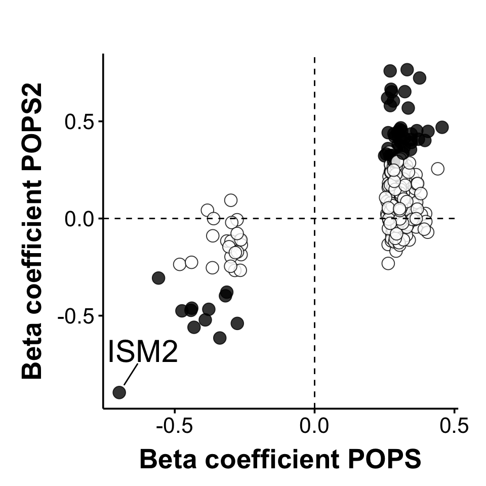
### Scatters of logistic regression beta coefficients for Composite 12wk-Fig.2j
```{r ,fig.width=5,fig.height=5,validation_POPS2_DAPs_Composite_12wk-all_line, message=FALSE, warning=FALSE}
log_X=lreg(data.frame(dl.npxz5.Roche.pops.composite.12wk%>%dplyr::select(-c(POPSID, Comparator,Roche_PlGF,Roche_PAPP_A,Roche_AFP,Roche_hCGbeta))
%>%dplyr::rename(y = last_col())), mc.cores=12)
log_Y=lreg(data.frame(dl.npxz5.pops2.composite.12wk%>%dplyr::select(-c(POPSID))%>%dplyr::rename(y = last_col())),mc.cores=12)
DAPs_X<- find_DEP(data.frame(dl.npxz5.Roche.pops.composite.12wk%>%dplyr::select(-c(POPSID, Comparator,Roche_PlGF,Roche_PAPP_A,Roche_AFP,Roche_hCGbeta))
%>%dplyr::rename(y = last_col())),  mc.cores=12,pvalue=0.05)
DAPs_Y<- find_DEP(data.frame(dl.npxz5.pops2.composite.12wk%>%dplyr::select(-c(POPSID))%>%dplyr::rename(y = last_col())),  mc.cores=12,pvalue=0.05)
merged_data <- inner_join(
  log_X %>%dplyr::select(feature, log_odds) %>% dplyr::rename(x = log_odds),
  log_Y %>% dplyr::select(feature, log_odds,pval) %>% dplyr::rename(y = log_odds),
  by = "feature")
data <- data.frame(
  features=merged_data$feature,
  x = merged_data$x,
  y = merged_data$y,
  color=merged_data$pval,
  re_color=log10(merged_data$pval) )
data$quadrant=ifelse(data$x>0 & data$y>0, 1,
                     ifelse(data$x>0  & data$y<0, 4,
                            ifelse(data$x<0  & data$y>0, 2, 3  )   ))
overlap=base::intersect(DAPs_X$feature,DAPs_Y$feature)
x_only=base::setdiff(DAPs_X$feature, DAPs_Y$feature)
y_only=base::setdiff(DAPs_Y$feature,DAPs_X$feature)
data$label <- ifelse(data$features %in% overlap, "overlap",
                     ifelse(data$features %in% x_only, "POPS_DAPs_only",
                            ifelse(data$features %in% y_only, "POPS2_DAPs_only", "non_DAPs")))
data= data %>%dplyr::filter(features %in% DAPs_X$feature)
data$features<- gsub("^NT\\.proBNP$", "NT-proBNP", data$features)
data$features <- gsub("^HLA\\.DRA$", "HLA-DRA", data$features)
data$features<- gsub("^HLA\\.E$", "HLA-E",data$features)
data$features<- gsub("^ERVV\\.1$", "ERVV-1",data$features)
data$features<- gsub("^HLA\\.A$", "HLA-A", data$features)
correlation_coefficient <- stats::cor(data$x, data$y, method = "spearman")
lm_model <- lm(y ~ x, data = data)
data$P_value <- ifelse(data$color < 0.05, "black", "white")
s4=ggplot(data, aes(x = x, y = y)) +
  geom_point(aes(fill = P_value), shape = 21, size = 4, stroke = 0.5, alpha = 0.8) +
  xlab("Beta coefficient POPS") +
  ylab("Beta coefficient POPS2") +
  ggtitle("") +
  geom_hline(yintercept = 0, linetype = "dashed", color = "black") +
  geom_vline(xintercept = 0, linetype = "dashed", color = "black") +
  theme(panel.background = element_rect(fill = "white")) +
  scale_fill_manual(values = c("black", "white"), labels = c("P < 0.05", "P ≥ 0.05")) +
  guides(fill = guide_legend(title = NULL)) +  # Hide legend title
    geom_text_repel(data = subset(data, features == "ISM2"), aes(label = features),
                  hjust = 0.8, vjust = 0.8, size = 8, color = "black",
                  nudge_y = 0.25, nudge_x = 0.15,
                  box.padding=0.2,point.padding=0.8,
                  segment.size = 0.5,segment.curvature = 0, direction = "y" ) +
   scale_x_continuous(breaks = c(-0.5, 0, 0.5, 1)) +
  scale_y_continuous(breaks = c(-0.5, 0, 0.5, 1)) +
  theme_Publication() +
    theme( legend.position = "none",
     panel.grid.major = element_blank(),
    panel.grid.minor = element_blank(),
    legend.title = element_blank(),
    axis.line = element_line(colour = "black"),
    axis.title = element_text(face = "bold", size = 20),
    axis.text = element_text(size = 16),
    plot.title = element_text(size = 20, face = "bold", hjust = 0.5),
    plot.margin = margin(0.5, 0.5, 0.5, 0.5, "cm"), ) +
  coord_fixed(ratio = 1) +   theme( aspect.ratio = 1  )
print(s4)
```
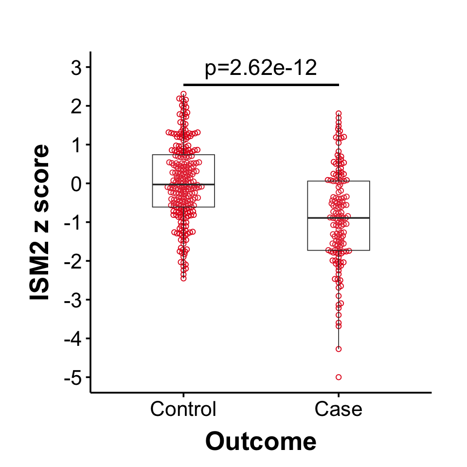
### Boxplot of GA adjusted z score of ISM2 12wkGA from the IMPACT study for complicated PE-Fig.2k
```{r ,fig.width=5,fig.height=5,sample-data-input, echo=FALSE, results='hide',message=FALSE, fig.show="hide"}
pheno <- read_excel("data/IMPACT_DATA_phenotypes_updated_v4.xlsx")
prot_all <- read.csv("data/IMPACT_DATA_Focus_NPXZ5_All.csv")
protein_name <- colnames(prot_all)[9] #"ISM2"
plgf_name <- colnames(prot_all)[15] #"PGF"
protein_display <- "ISM2"
outcome_cols <- c("PE_all", "PE_pt_all", "PE_t_all", "PE_FGR_all", "PE_noFGR_all")
outcome_labels <- c("PE (all)", "PE (preterm)", "PE (term)",
"PE with FGR", "PE without FGR")
dat_all <- merge(prot_all, pheno, by = "SampleID")
#Parity == 1: Nulliparous
dat_nullip <- dat_all[dat_all$Parity == 1, ]
##Parity == 0: parous
dat_parous <- dat_all[dat_all$Parity == 0, ]
datasets <- list(Nulliparous = dat_nullip, All = dat_all, Parous = dat_parous)
pop_labels <- names(datasets)
count_cases <- function(dat, oc) {
x <- dat[[oc]]
x <- as.numeric(x[!is.na(x) & x != ""])
sum(x == 1, na.rm = TRUE)
}
summary_df <- data.frame(
Population = pop_labels,
n = sapply(datasets, nrow)
)
for (i in seq_along(outcome_cols)) {
summary_df[[outcome_labels[i]]] <- sapply(datasets, count_cases, oc = outcome_cols[i])
}
```
```{r fig2k_paper,fig.width=5, fig.height=5,message=FALSE, warning=FALSE}
df <- datasets$All
df <- df[!is.na(df$ISM2) & !is.na(df$PE_all), ]
df$group <- factor(df$PE_all,
                   levels = c(0,1),
                   labels = c("Control","Case"))
df_plot <- df[, c("ISM2", "PE_all", "group")]
shapiro_control <- shapiro.test(df$ISM2[df$group == "Control"])
shapiro_case <- shapiro.test(df$ISM2[df$group == "Case"])
if (shapiro_control$p.value > 0.05 & shapiro_case$p.value > 0.05) {
  test_res <- t.test(ISM2 ~ group, data = df, var.equal = F)
  test_name <- "t-test"
} else {
  test_res <- wilcox.test(ISM2 ~ group, data = df)
  test_name <- "Wilcoxon"
}
p_value <- test_res$p.value
p_value_fmt <- formatC(p_value, format = "e", digits = 2)
p_label <- paste0("p=", p_value_fmt)
y_max <- max(df$ISM2, na.rm = TRUE)
y_line <- y_max * 1.10
y_text <- y_max * 1.3
ggplot(df, aes(x = group, y = ISM2)) +
  geom_beeswarm(color = "#E31A1C", cex = 0.9, shape = 1) +
  geom_boxplot(
    aes(group = group),
    alpha = 0.1,
    outlier.shape = NA,
    width = 0.4,
    linewidth = 0.3
  ) +
  geom_segment(
    aes(x = 1, xend = 2, y = y_line, yend = y_line),
    inherit.aes = FALSE,
    size = 0.8
  ) +
  annotate(
    "text",
    x = 1.5,
    y = y_text,
    label = p_label,
    size = 6
  ) +
  labs(
    title = " ",
    x = "Outcome",
    y = "ISM2 z score"
  ) +
  scale_y_continuous(breaks = seq(-5, 3, by = 1)) +
  theme_Publication() +
  theme(
    panel.grid.major = element_blank(),
    panel.grid.minor = element_blank(),
    legend.position = "none",
    axis.line = element_line(colour = "black"),
    axis.title = element_text(face = "bold", size = 20),
    axis.text = element_text(size = 16),
    plot.title = element_text(size = 20, face = "bold", hjust = 0.5),
    plot.margin = margin(0.5, 0.5, 0.5, 0.5, "cm"),
    aspect.ratio = 1
  ) +
  coord_fixed(ratio = 1)
```
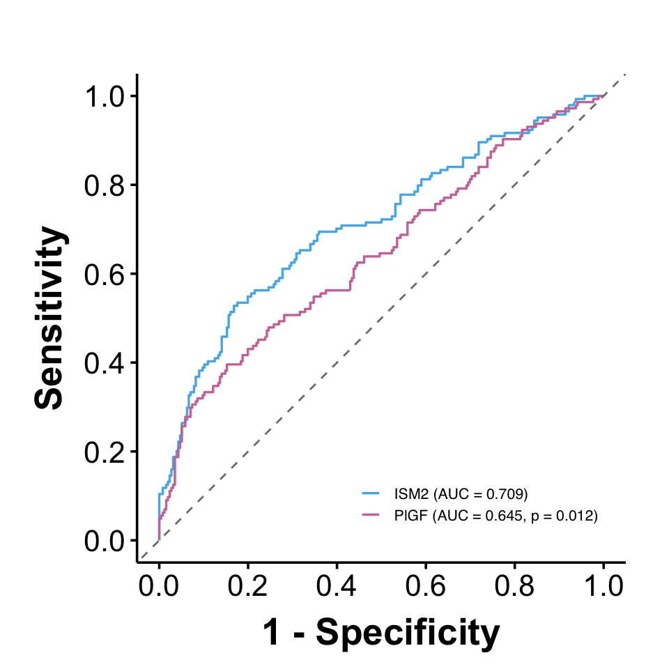
### ROC curve plots of ISM2 and PlGF from the IMPACT study for complicated PE-Fig.2l
```{r roc-pe-all-format_V3,fig.width=5, fig.height=5,message=FALSE, warning=FALSE}
t_all  <- table(factor(datasets$All$PE_all, levels = c(0, 1)))
plot_roc_V3 <- function(data, protein_col, plgf_col, outcome_col, title) {
  condition_colors <- c(
    "ISM2" = "#56B4E9",
    "PlGF" = "#CC79A7" )
  df <- data %>%
    dplyr::select(all_of(c(protein_col, plgf_col, outcome_col))) %>%
    dplyr::rename(y = all_of(outcome_col)) %>%
    drop_na()
  fit_ism2 <- glm(y ~ ., data = df[, c("y", protein_col)], family = binomial)
  fit_plgf <- glm(y ~ ., data = df[, c("y", plgf_col)], family = binomial)
  df$pred_ism2 <- fitted(fit_ism2)
  df$pred_plgf <- fitted(fit_plgf)
  roc_ism2 <- roc(df$y, df$pred_ism2, quiet = TRUE)
  roc_plgf <- roc(df$y, df$pred_plgf, quiet = TRUE)
  delong_p <- roc.test(roc_ism2, roc_plgf, method = "delong")$p.value
  label_ism2 <- sprintf("ISM2 (AUC = %.3f)", auc(roc_ism2))
  label_plgf <- sprintf("PlGF (AUC = %.3f, p = %.3f)", auc(roc_plgf), delong_p)
  roc_df <- rbind(
    data.frame(
      Specificity = roc_ism2$specificities,
      Sensitivity = roc_ism2$sensitivities,
      Protein = "ISM2",
      Label = label_ism2    ),
    data.frame(
      Specificity = roc_plgf$specificities,
      Sensitivity = roc_plgf$sensitivities,
      Protein = "PlGF",
      Label = label_plgf
    )  )
  roc_df <- roc_df %>%
  dplyr::distinct(Protein, Specificity, Sensitivity, .keep_all = TRUE) %>%
  dplyr::arrange(Protein, Specificity, Sensitivity)
  ggplot(roc_df, aes(x = 1 - Specificity, y = Sensitivity,
                     color = Protein, linetype = Protein)) +
    geom_step(size = 0.6, direction = "hv") +
    geom_abline(slope = 1, intercept = 0,
                linetype = "dashed", color = "gray50") +
    labs(title = title,
         x = "1 - Specificity",
         y = "Sensitivity") +
    scale_x_continuous(limits = c(0, 1), breaks = seq(0, 1, 0.2)) +
    scale_y_continuous(limits = c(0, 1), breaks = seq(0, 1, 0.2)) +
    scale_color_manual(values = condition_colors,
                       labels = c(label_ism2, label_plgf)) +
    scale_linetype_manual(values = c("ISM2" = "solid", "PlGF" = "solid"),
                          labels = c(label_ism2, label_plgf)) +
    theme_Publication() +
    theme(
      legend.position = c(0.7, 0.12),#  legend.position = "none",
      legend.title = element_blank(),
      legend.text = element_text(size = 8),
      legend.key.size = unit(0.8, "lines"),
      panel.grid.major = element_blank(),
      panel.grid.minor = element_blank(),
      axis.line = element_line(colour = "black"),
      axis.title = element_text(face = "bold", size = 20),
      axis.text = element_text(size = 16),
      plot.title = element_text(size = 20, face = "bold", hjust = 0.5),
      plot.margin = margin(0.5, 0.5, 0.5, 0.5, "cm"),
      aspect.ratio = 1
    ) +
    coord_fixed(ratio = 1)
}
plot_roc_V3(datasets$All,"ISM2","PGF","PE_all"," ")
```