# Supplementary Text Figures {#sec-suppl-figure}
This chapter demonstrates the `R` codes that make supplementary text figures shown in the paper.
Making the main figures are shown in @sec-main-figure.
## Supplementary Text Figure 1 {#sec-si-fig1}
### Supplementary Text Figure 1A {#sec-si-fig1a}
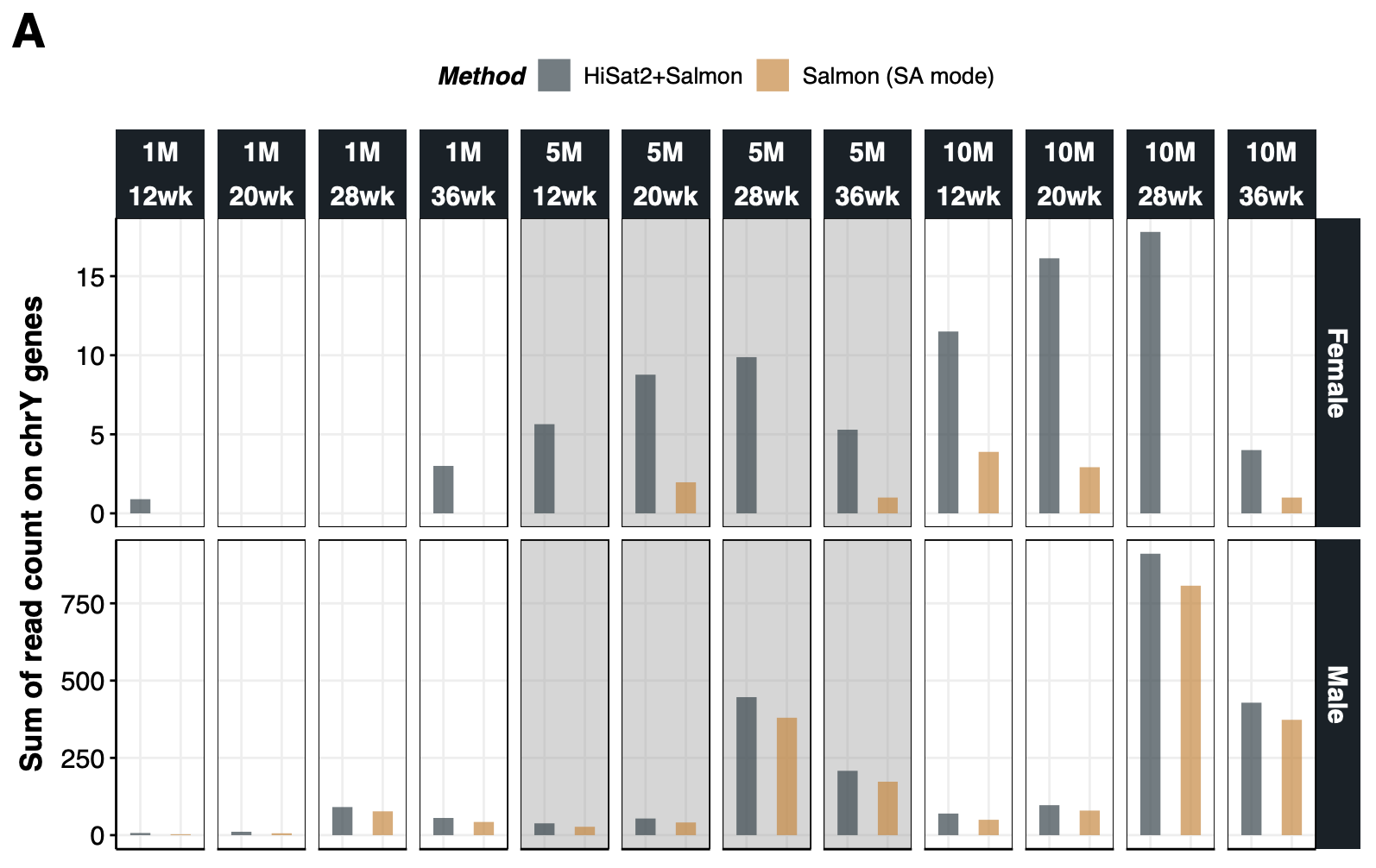{#fig-si-fig1a}
```{r }
#| label: si-fig-1a
#| eval: false
  lazyLoad("downsample.chrY.TPM_cache/beamer/load_ds_salmon_4b8dd727729fd0ae5deb423d69e7c16d") # dl.chrY.TPM and dl.stat

  dt.ds.chrY <- lapply(names(dl.stat), function(DS) dl.stat[[DS]][,DS:=DS]) %>% rbindlist
  dt.ds.chrY$DS<-factor(dt.ds.chrY$DS, level=c("1M","5M","10M"))
  dt.ds.chrY[,GA:=gsub(" weeks","wk",GA)]
  setnames(dt.ds.chrY, "Type", "Method")

  p1.chrY<-ggplot(dt.ds.chrY, aes(Method,SumCount)) +
  geom_rect(data = dt.ds.chrY[DS=="5M"],fill="grey60",xmin = -Inf,xmax = Inf, ymin = -Inf,ymax = Inf,alpha = 0.2) +
  geom_bar(aes(fill=Method), stat="identity",width=.5, alpha=.7) +
  ggsci::scale_fill_jama() +
  facet_grid(Sex~DS+GA,scales="free") +
  labs(y="Sum of read count on chrY genes") +
  theme_Publication() +
  theme(legend.position="top",
        panel.border=element_rect(colour="black"),
        axis.title.x=element_blank(),
        axis.text.x=element_blank(),
        axis.ticks.x=element_blank())

  #
  pdf(file="Figures/Suppl/cfRNA.Suppl.Text.Fig1A.pdf", width=11, height=8, title="Abundance of chrY")
  p1.chrY
  dev.off()
```
### Supplementary Text Figure 1B {#sec-si-fig1b}
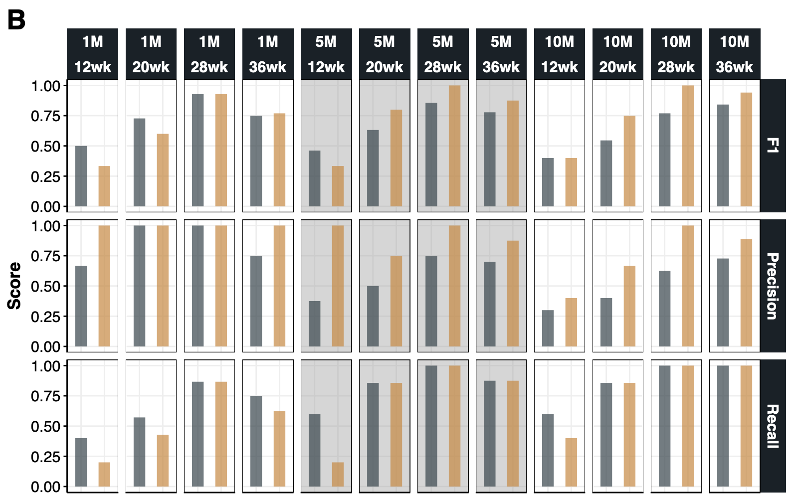{#fig-si-fig1b}
```{r }
#| label: si-fig-1b
#| eval: false
  lazyLoad("downsample.chrY.TPM_cache/beamer/load_ds_salmon_4b8dd727729fd0ae5deb423d69e7c16d") # dl.chrY.TPM and dl.stat

  lapply(dl.chrY.TPM, function(i) i[,.(sum(Counts),sum(TPM))])

  dl.chrY.TPM<-lapply(dl.chrY.TPM, function(DT) {
                  #DT[Sex=="Male",Class:=ifelse(TPM>0,"TP","FN")]
                  #DT[Sex=="Female",Class:=ifelse(TPM==0,"TN","FP")]
                  DT[,`Predicted Sex`:=ifelse(TPM>0, "Male","Female"),Type]
                  DT$Sex<-factor(DT$Sex, level=c("Male","Female"))
                  DT$`Predicted Sex`<-factor(DT$`Predicted Sex`, level=c("Male","Female"))
                  DT
  })

  #####################################
  # Predictive performance by DS & GA #
  #####################################
  dt.chrY.con.ga<-lapply(names(dl.chrY.TPM), function(DS){
    lapply(split(dl.chrY.TPM[[DS]], dl.chrY.TPM[[DS]]$GA), function(DT){
    my.GA<-DT[,.N,GA]$GA

    cm1<-caret::confusionMatrix(DT[Type=="HiSat2+Salmon"][["Predicted Sex"]], reference=DT[Type=="HiSat2+Salmon"][["Sex"]])
    cm2<-caret::confusionMatrix(DT[Type=="Salmon (SA mode)"][["Predicted Sex"]], reference=DT[Type=="Salmon (SA mode)"][["Sex"]])

    rbind(
    data.table(DS=DS, GA=my.GA,Type="HiSat2+Salmon", Measure=names(cm1$byClass), Value=cm1$byClass),
    data.table(DS=DS, GA=my.GA,Type="Salmon (SA mode)", Measure=names(cm2$byClass), Value=cm2$byClass)
    )[Measure %in% c("F1","Precision", "Recall")]
    }) %>% rbindlist
  }) %>% rbindlist

  dt.chrY.con.ga$DS<-factor(dt.chrY.con.ga$DS, level=c("1M","5M","10M"))
  dt.chrY.con.ga[,GA:=gsub(" weeks","wk",GA)]
  setnames(dt.chrY.con.ga, "Type", "Method")

  p1.chrY.con<-ggplot(dt.chrY.con.ga, aes(Method,Value)) +
  geom_rect(data = dt.chrY.con.ga[DS=="5M"],fill="grey60",xmin = -Inf,xmax = Inf, ymin = -Inf,ymax = Inf,alpha = 0.2) +
  geom_bar(aes(fill=Method), stat="identity",width=.5, alpha=.7) +
  ggsci::scale_fill_jama() +
  facet_grid(Measure~DS+GA,scales="free") +
  labs(y="Score") +
  theme_Publication() +
  theme(legend.position="none",
        panel.border=element_rect(colour="black"),
        axis.title.x=element_blank(),
        axis.text.x=element_blank(),
        axis.ticks.x=element_blank())


  # merge SI.Fig1A + SI.Fig1B
  pdf(file="Figures/Suppl/cfRNA.Suppl.Text.Fig1AB.pdf", width=11, height=14, title="Abundance of chrY")
  cowplot::plot_grid(p1.chrY, p1.chrY.con, labels="AUTO", ncol=1, label_size=27, align="v", axis="l")
  dev.off()
```
### Supplementary Text Figure 1C {#sec-si-fig1c}
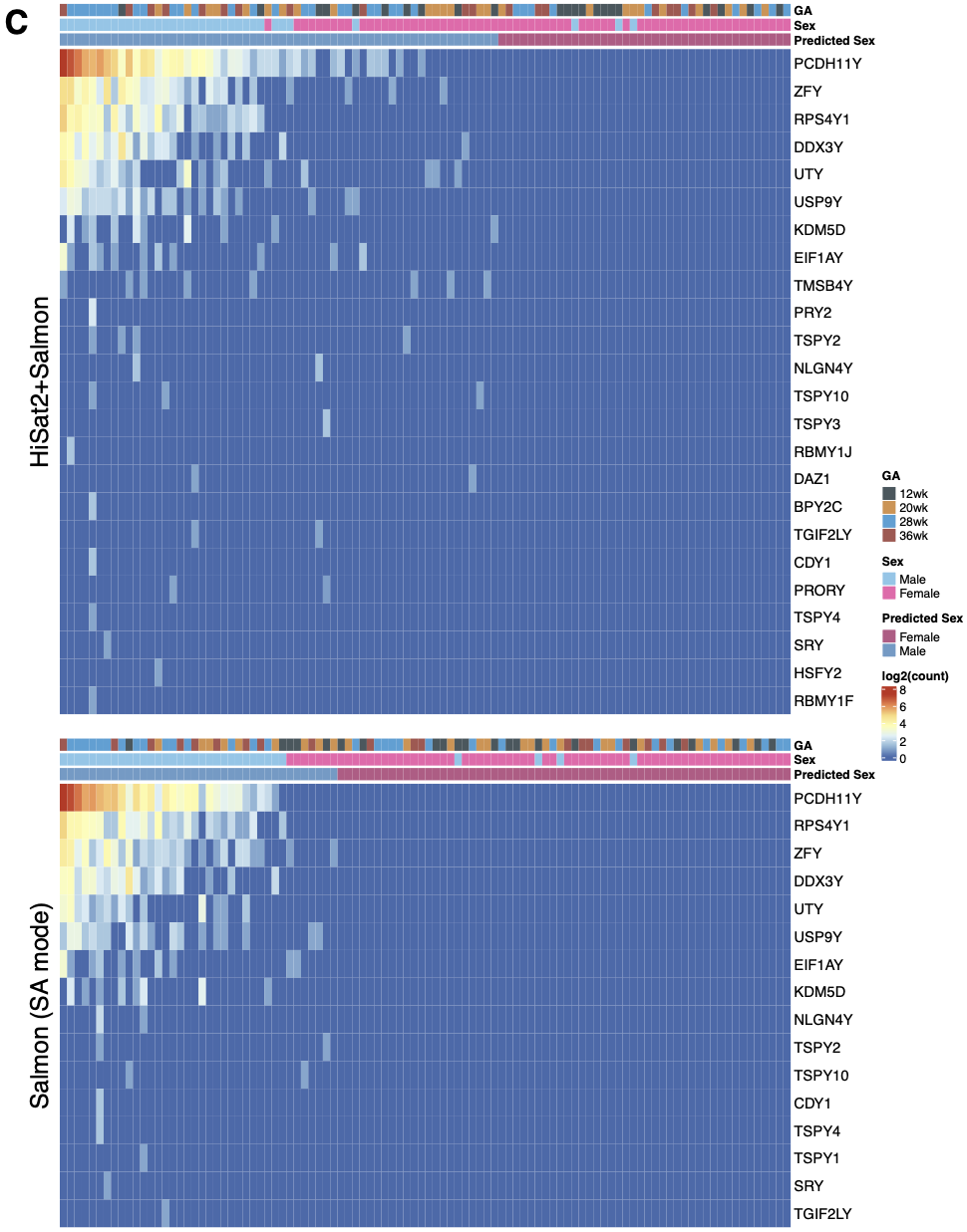{#fig-si-fig1c}
```{r }
#| label: si-fig-1c
#| eval: false
  # load the transcript definition used in Salmon (SA)
  load("RData/gr.ensg.Homo_sapiens.GRCh38.88.cdna.all.ncrna.fa.gz.RData") %>% system.time # isa GRanges
  gr.ensg[seqnames(gr.ensg)=="Y" & gr.ensg$gene_biotype=="protein_coding",] # chrY protein-coding; n=42
  this.gene<-(gr.ensg[seqnames(gr.ensg)=="Y" & gr.ensg$gene_biotype=="protein_coding",] %>% names) # chrY protein-coding; n=42 (without the training version e.g. ENSG00000176679)

  # load the TPM based om 10M-ds dataset
  load("RData/li.TPM.10M.RData")
  li.TPM[["Salmon_aln"]][["TPM"]] %>% dim # 62803 genes x 100 samples

  ## Heatamp of TPM using `HiSat2+Salmon` (based on 10M)
  li.TPM[["Salmon_aln"]][["counts"]][this.gene,] %>% rowSums %>% sort %>% rev # count of 42 chrY genes
  filter.g2<-li.TPM[["Salmon_aln"]][["counts"]][this.gene,] %>% rowSums %>% sort %>% rev >0 # filter for 42 chrY genes with TPM >0
  this.gene2<-(li.TPM[["Salmon_aln"]][["counts"]][this.gene,] %>% rowSums %>% sort %>% rev)[filter.g2] %>% names # n=24 genes
  this.sample2<-li.TPM[["Salmon_aln"]][["counts"]][this.gene,] %>% colSums %>% sort %>% rev %>% names # n=100 samples sorted
  filter.s2<-li.TPM[["Salmon_aln"]][["counts"]][this.gene2,] %>% colSums %>% sort %>% rev >0 # filter for samples with TPM >0
  predicted.male2<-(li.TPM[["Salmon_aln"]][["counts"]][this.gene,] %>% colSums %>% sort %>% rev)[filter.s2] %>% names # n=60 samples

  my.mat2<-log2(li.TPM[["Salmon_aln"]][["counts"]][this.gene2,this.sample2]+1)
  rownames(my.mat2)<-gr.ensg[this.gene2]$gene_name

  col.anno<-mat.samples[this.sample2,c("GA","Sex"),drop=F] # isa `data.frame`
  col.anno$"Predicted Sex"<-ifelse(this.sample2 %in% predicted.male2,"Male","Female")
  col.anno<-col.anno[,c("Predicted Sex","Sex","GA")]

  GA.color<-ggsci::pal_jama("default",alpha=.9)(4)
  names(GA.color)<-c("12wk","20wk","28wk","36wk")
  my.color=list(
      `Sex`=c(Female="hotpink",Male='skyblue'),
      `Predicted Sex`=c(Female="hotpink3",Male='skyblue3'),
      #`GA`=c("12wk"=cbPalette2[1],"20wk"=cbPalette2[2],"28wk"=cbPalette2[3],"36wk"=cbPalette2[4])
      `GA`=GA.color
  )

  cph1<-ComplexHeatmap::pheatmap(my.mat2,
                                 annotation_col=col.anno,
                                 annotation_colors=my.color,
                                 cluster_cols=F,
                                 cluster_rows=F,
                                 show_colnames=F,
                                 border_color=NA,
                                 fontsize=12,
                                 name="log2(count)",
                                 row_title="\nHiSat2+Salmon",
                                 row_title_gp = gpar(fontsize = 20),
  )

  filter.g3<-li.TPM[["Salmon"]][["counts"]][this.gene,] %>% rowSums %>% sort %>% rev >0 # filter for 42 chrY genes with count >0
  this.gene3<-(li.TPM[["Salmon"]][["counts"]][this.gene,] %>% rowSums %>% sort %>% rev)[filter.g3] %>% names # n=16 genes (out of 42) >0 count
  this.sample3<-li.TPM[["Salmon"]][["counts"]][this.gene,] %>% colSums %>% sort %>% rev %>% names # 100 sample names
  filter.s3<-li.TPM[["Salmon"]][["counts"]][this.gene3,] %>% colSums %>% sort %>% rev >0 # samples with count>0
  #(li.TPM[["Salmon"]][["counts"]][this.gene,] %>% colSums %>% sort %>% rev)[filter.s3] # n=38 samples with count>0 (predicted as Male)
  predicted.male3<-(li.TPM[["Salmon"]][["counts"]][this.gene,] %>% colSums %>% sort %>% rev)[filter.s3] %>% names # n=38 samples with count>0 (predicted as Male)

  my.mat3<-log2(li.TPM[["Salmon"]][["counts"]][this.gene3,this.sample3]+1)
  rownames(my.mat3)<-gr.ensg[this.gene3]$gene_name

  col.anno3<-mat.samples[this.sample3,c("GA","Sex"),drop=F]
  col.anno3$"Predicted Sex"<-ifelse(this.sample3 %in% predicted.male3,"Male","Female")
  col.anno3<-col.anno3[,c("Predicted Sex","Sex","GA")]

  # via ComplexHeatmap
  cph3<-ComplexHeatmap::pheatmap(my.mat3,
                                 annotation_col=col.anno3,
                                 annotation_colors=my.color,
                                 cluster_cols=F,
                                 cluster_rows=F,
                                 show_colnames=F,
                                 border_color=NA,
                                 fontsize=12,
                                 name="log2(count)",
                                 row_title="\nSalmon (SA mode)",
                                 row_title_gp = gpar(fontsize = 20),
                                 heatmap_legend_param = list(
                                                            title_gp=gpar(fontsize=13,fontface="bold"),
                                                            labels_gp=gpar(fontsize=11),
                            annotation_legend_param = list(title_gp=gpar(fontsize=13,fontface="bold"),labels_gp = gpar(fontsize = 11))
                                )
  )


  pdf(file="Figures/Suppl/cfRNA.Suppl.Text.Fig1C.pdf", width=11, height=14, title="Abundance of chrY")
  draw(cph1 %v% cph3, main_heatmap="log2(count)", ht_gap=unit(.7,"cm"), auto_adjust=F)
  grid.text(label="C",gp=gpar(fontsize=27,fontface="bold"),x=0.02,y=.99,just="top")
  dev.off()
```
### Supplementary Text Figure 1D {#sec-si-fig1d}
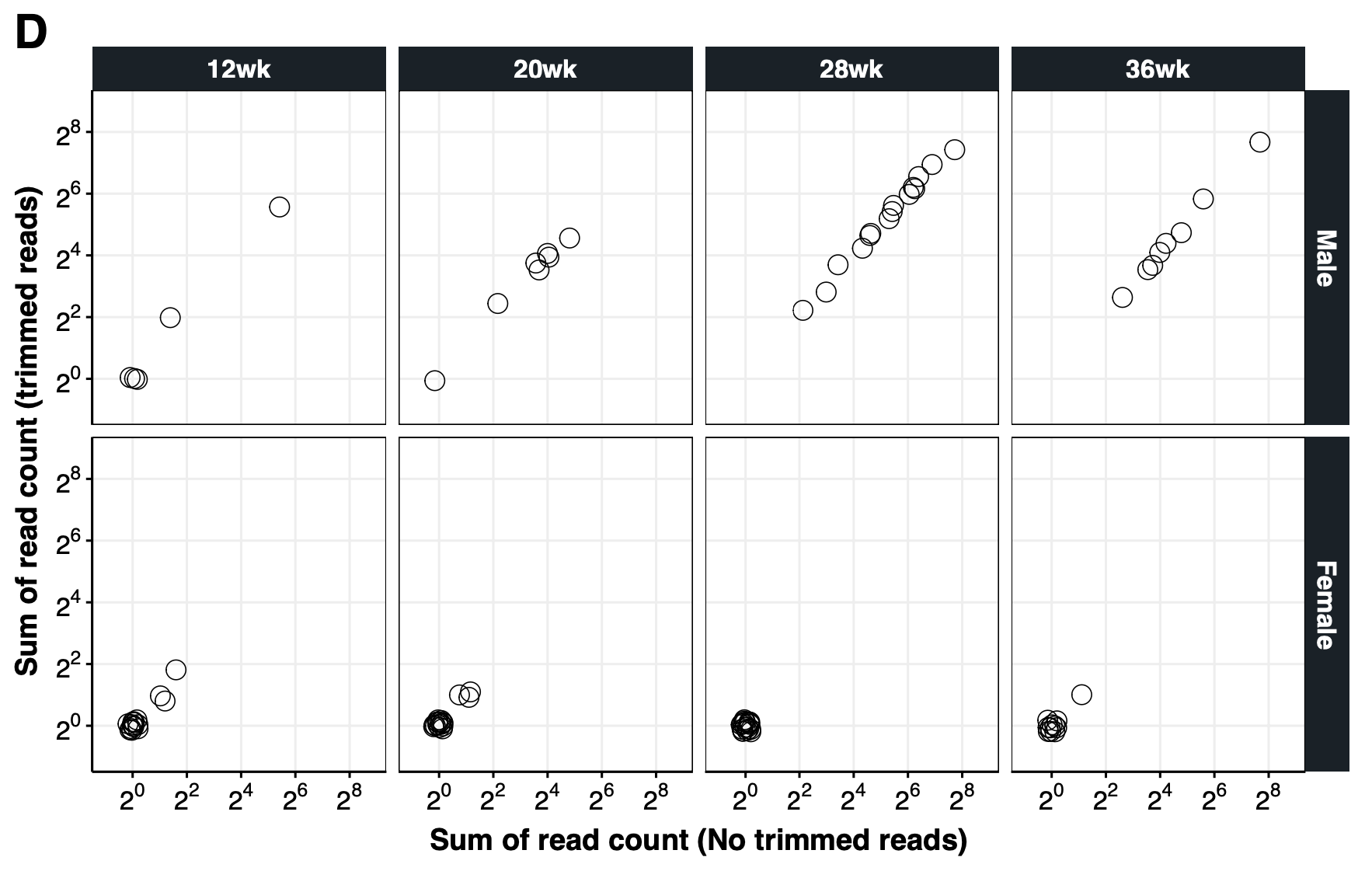{#fig-si-fig1d}
```{r }
#| label: si-fig-1d
#| eval: false
  dl.chrY.TPM %>% names

  # load the TPM based om 10M-ds dataset
  load("RData/li.TPM.10M.trim.RData")
  li.TPM[["Salmon"]][["TPM"]] %>% dim # 59354 genes x 100 samples

  dt.trim.10M<-data.table(
      `Type`="Salmon (SA mode)",
      `SampleID`=li.TPM[["Salmon"]][["counts"]][this.gene,] %>% colSums %>% names,
      `Counts`=li.TPM[["Salmon"]][["counts"]][this.gene,] %>% colSums,
      `TPM`=li.TPM[["Salmon"]][["TPM"]][this.gene,] %>% colSums
      )
  # add Sex and GA
  dt.trim.10M<-merge(dt.trim.10M, dt.samples[,.(SampleID,GA,Sex,pn_female)])

  dt.trim.10M[,`Predicted Sex`:=ifelse(TPM>0, "Male","Female"),Type]
  dt.trim.10M$Sex<-factor(dt.trim.10M$Sex, level=c("Male","Female"))
  dt.trim.10M$`Predicted Sex`<-factor(dt.trim.10M$`Predicted Sex`, level=c("Male","Female"))

  dt.chrY.trim<-rbind(
        dl.chrY.TPM[["10M"]][Type=="Salmon (SA mode)"][,Trim:="No"],
        dt.trim.10M[,Trim:="Yes"]
        )
  ## Number of false positives: chrY signal detected from females
  dt.chrY.trim[,.(Trim,Sex,`Predicted Sex`)] %>% ftable

  ##
  ## Read counts by trim or not
  dt.bar<-merge(
    dl.chrY.TPM[["10M"]][Type=="Salmon (SA mode)",.(SampleID,GA=gsub(" weeks","wk",GA),Sex,Counts,TPM)], # no-trim
    dt.trim.10M[Type=="Salmon (SA mode)",.(SampleID,GA,Sex,Counts,TPM)], # trim
    by=c("SampleID","Sex","GA")
  )
  cor.test(~Counts.x + Counts.y, dt.bar)
  dt.bar[Counts.x>Counts.y] # no-trim > trim
  dt.bar[Counts.x<Counts.y] # no-trim < trim
  dt.bar[Sex=="Female" & Counts.x<Counts.y] # more counts for Trimmed Salmon

  my.limit<-dt.bar[,max(Counts.x,Counts.y)]  %>% ceiling
  p1.chrY.trim<-ggplot(dt.bar, aes(Counts.x+1,Counts.y+1)) +
  geom_point(data=dt.bar, size=5, position=position_jitter(width=0.2,height=0.2),shape=21) +
  scale_x_continuous(trans = scales::log2_trans(),
                     breaks = scales::trans_breaks("log2",function(x) 2^x),
                     labels = scales::trans_format("log2", math_format(2^.x)),
                     limits=c(.5,my.limit*2)) +
  scale_y_continuous(trans = scales::log2_trans(),
                     breaks = scales::trans_breaks("log2",function(x) 2^x),
                     labels = scales::trans_format("log2", math_format(2^.x)),
                     limits=c(.5,my.limit*2)) +
  #coord_fixed() +
  facet_grid(Sex~GA,scales="free_x") +
  labs(x="Sum of read count (No trimmed reads)", y="Sum of read count (trimmed reads)") +
  theme_Publication() + theme(panel.border = element_rect(colour = "black"))

  pdf(file="Figures/Suppl/cfRNA.Suppl.Text.Fig1D.v2.pdf", width=11, height=7, title="Trim vs No trim")
  cowplot::plot_grid(p1.chrY.trim, labels=c("D"),label_size=27)
  dev.off()
```
## Supplementary Text Figure 2 {#sec-si-fig2}
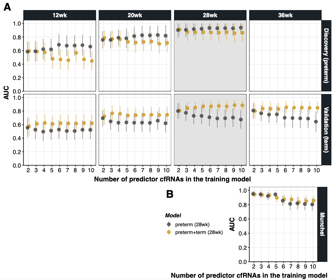{#fig-si-fig2}
```{r}
#| label: si-fig2
#| eval: false
load("RData/dl.enet.result.core17.RData") # Validation of ENet models from 28wk, discovery dataset (preterm)
load("RData/dl.combined.result.core17.RData") # Validation of ENet models from the combined model (preterm+term)

##
## AUC in All
##
ga<-paste0(c(12,20,28,36), "wk")
term<-c("(preterm)","(term)")
my.dataset<-data.table(expand.grid(ga,term))[,Var3:=paste0(Var1,Var2)][Var3!="36wk(preterm)"]$Var3
my.dataset<-c("Munchel",my.dataset)

dt.auc.long<-
lapply(my.dataset, function(this.dataset){
  rbind(
        (lapply(2:10, function(my.num) dl.combined.result[[my.num-1]][fold==this.dataset,.(Num=my.num,Predictor=predictor,AUC_test=AUC_test/100,AUC_test_lo=AUC_test_lo/100,AUC_test_hi=AUC_test_hi/100)]) %>% rbindlist)[,Model:="preterm+term (28wk)"]
        ,
        (lapply(2:10, function(my.num) dl.enet.result[[my.num-1]][fold==this.dataset & grepl("ENet",methods),.(Num=my.num,Predictor=predictor,AUC_test=AUC_test/100,AUC_test_lo=AUC_test_lo/100,AUC_test_hi=AUC_test_hi/100)]) %>% rbindlist)[,Model:="preterm (28wk)"]

  )[,Dataset:=this.dataset]
}) %>% rbindlist %>% setcolorder(c("Dataset","Model"))

dt.auc.long[Dataset!="Munchel",GA:=substr(Dataset,1,4)]
dt.auc.long[Dataset!="Munchel",Source:=substr(Dataset,6,nchar(Dataset)-1)][,Source:=ifelse(Source=="preterm","Discovery (preterm)","Validation (term)")]
dt.auc.long[Dataset=="Munchel",`:=`(Source="Munchel",GA="36wk")]
dt.auc.long$Model<-factor(dt.auc.long$Model, level=c("preterm (28wk)","preterm+term (28wk)"))
dt.auc.long$Source<-factor(dt.auc.long$Source, level=c("Discovery (preterm)","Validation (term)","Munchel"))

p.auc.combined.A<-ggplot(dt.auc.long[Source!="Munchel"], aes(Num, AUC_test,group=Model)) +
  geom_rect(data = dt.auc.long[Source!="Munchel" & GA=="28wk"],aes(fill = GA),fill="grey90",xmin = -Inf,xmax = Inf, ymin = -Inf,ymax = Inf,alpha = 0.2) +
  geom_pointrange(aes(col=Model,ymin=AUC_test_lo, ymax=AUC_test_hi),
                  position=position_dodge(width=0.4),
                  size=.8,alpha=.8) +
  scale_y_continuous(expand=c(0,0),breaks=c(0,.2,.4,.6,.8,1), limit=c(0,1.05)) +
  scale_x_continuous(breaks=2:10) +
  labs(y="AUC", x="Number of predictor cfRNA in the training model") +
  scale_color_manual(values=c("grey30",cbPalette2[2])) +
  facet_grid(Source~GA) +
  theme_Publication() +
  theme(legend.position="", panel.border = element_rect(colour = "black"))

p.auc.combined.B<-ggplot(dt.auc.long[Source=="Munchel"], aes(Num, AUC_test,group=Model)) +
  geom_pointrange(aes(col=Model,ymin=AUC_test_lo, ymax=AUC_test_hi),
                  position=position_dodge(width=0.4),
                  size=.8,alpha=.8) +
  scale_y_continuous(expand=c(0,0),breaks=c(0,.2,.4,.6,.8,1), limit=c(0,1.05)) +
  scale_x_continuous(breaks=2:10) +
  labs(y="AUC", x="Number of predictor cfRNA in the training model                                     ") +
  scale_color_manual(values=c("grey30",cbPalette2[2])) +
  facet_grid(Source~.) +
  theme_Publication() +
  theme(legend.position="left",
        panel.border = element_rect(colour = "black"),
        plot.margin=margin(1,-15,7,0)
  )

p.auc.bottom<-cowplot::plot_grid(NULL,p.auc.combined.B, nrow=1,labels=c("","B"),label_size=27,rel_widths=c(.87,1))

pdf(file="Figures/Suppl/cfRNA.Suppl.Data.Fig.combined.AUC.AB.pdf", width=12, height=10, title="Suppl Fig: AUC from the combined model vs preterm model")
cowplot::plot_grid(p.auc.combined.A, p.auc.bottom,ncol=1, labels=c("A",""),label_size=27,rel_heights=c(2,1), align="v", axis="lr")
dev.off()
```
## Supplementary Text Figure 3 {#sec-si-fig3}
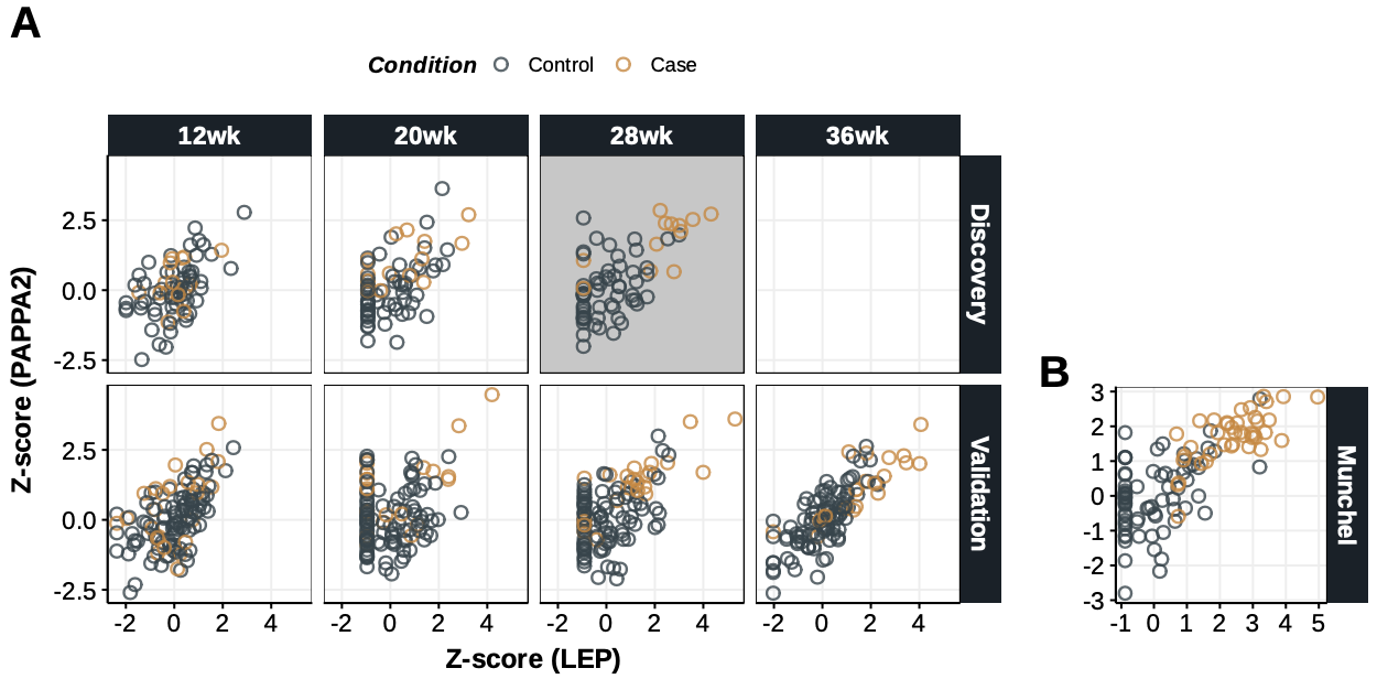{#fig-si-fig3}
```{r}
#| label: si-fig3
#| eval: false
load("RData/dt.cpmZ.preterm.POPS-2022.GRCh38.88.RData") # dt.cpmZ (preterm)
load("RData/dt.cpmZ.term.POPS-2022.GRCh38.88.RData") # dt.cpmZ.term (term)
load("RData/dt.cpmZ.munchel.RData") # dt.cpmZ.munchel (Munchel)

dt.lep.pappa2<-rbind(
                      (dt.cpmZ[geneName %in% c("LEP","PAPPA2")] %>% dcast.data.table(SampleID+GA+Condition~geneName, value.var="logCPMZ"))[,Source:="Discovery"],
                      (dt.cpmZ.term[geneName %in% c("LEP","PAPPA2")] %>% dcast.data.table(SampleID+GA+Condition~geneName, value.var="logCPMZ"))[,Source:="Validation"],
                      (dt.cpmZ.munchel[geneName %in% c("LEP","PAPPA2")] %>% dcast.data.table(SampleID+Condition~geneName, value.var="logCPMZ"))[,Source:="Munchel"]
    ,fill=T)

dt.lep.pappa2[,Dataset:=ifelse(is.na(GA),Source,paste0(Source,"(",GA,")"))]
dt.lep.pappa2[,.(Cor=cor(LEP,PAPPA2),Pval=cor.test(LEP,PAPPA2)$p.value),.(Source,GA)][order(Source,GA)]
dt.lep.pappa2[Condition=="Case",.(Cor=cor(LEP,PAPPA2),Pval=cor.test(LEP,PAPPA2)$p.value),.(Source,GA)][order(Source,GA)]

p1<-
ggplot(dt.lep.pappa2[Source!="Munchel"], aes(LEP,PAPPA2)) +
  geom_rect(data = dt.lep.pappa2[Source=="Discovery" & GA=="28wk"],aes(fill = GA),fill="grey80",xmin = -Inf,xmax = Inf, ymin = -Inf,ymax = Inf,alpha = 0.2) +
  geom_point(aes(col=Condition),size=3,shape=21,stroke=1.1,alpha=.8) +
  facet_grid(Source~GA) +
  ggsci::scale_color_jama() +
  labs(x="Z-score (LEP)",y="Z-score (PAPPA2)") +
  theme_Publication() +theme (panel.border = element_rect(colour = "black"),legend.position="top")

p2<-
ggplot(dt.lep.pappa2[Source=="Munchel"], aes(LEP,PAPPA2)) +
  geom_point(aes(col=Condition),size=3,shape=21,stroke=1.1,alpha=.8) +
  facet_grid(Source~.) +
  ggsci::scale_color_jama() +
  labs(x="",y="") +
  theme_Publication() +theme (panel.border = element_rect(colour = "black"),legend.position="")

p2.right<-cowplot::plot_grid(NULL,p2,labels=c("","B"),ncol=1,label_size=27,rel_heights=c(1,1))
p.corr2<-cowplot::plot_grid(p1, p2.right, labels=c("A",""),label_size=27,rel_widths=c(2.8,1))

cairo_pdf(file="Figures/Suppl/cfRNA.Suppl.LEP.PAPPA2.cor2.pdf", width=12,height=6, onefile=T)
p.corr2
dev.off()
```
## Supplementary Text Figure 4, 5, and 6 {#sec-si-fig4-6}
{width=100% height=475px}
[Full Screen](static/figure/cfRNA.SI.Fig4.5.6.pdf)
You may need to refer to @sec-ga-long and @sec-fig5b
```{r rlmer_csh1_plot}
#| label: si-fig456
#| eval: false
targets<-c(
  dt.R2.GA2[order(-r2m)][["gene"]][1:100], # top 100 by r2
  dt.R2.GA2[order(p.combined)][["gene"]][1:100], # top 100 by the combined p-value
  dt.R2.GA[BH.GA<0.05][order(p.GA)][coef.GA<0][["gene"]][1:100] # top 100 decreasing
  ) %>% unique
#
li.plots<-lapply(dl.logCPM[targets], function(dt.foo){
    my.gene<-unique(dt.foo[["geneName"]])
    message(my.gene)

    r2m<-li.lmer[[my.gene]][["stat"]][Model=="GA2"][["r2m"]] %>% round(3)
    r2c<-li.lmer[[my.gene]][["stat"]][Model=="GA2"][["r2c"]] %>% round(3)
    #my.title=paste0(my.gene," (r2m:",r2m,", r2c:",r2c,")")
    my.title=paste0(my.gene," (r2m:",r2m,")")

    my.title.y<-latex2exp::TeX(r"($\textbf{log_2 CPM}$)")

    ggplot(dt.foo, aes(x = GAwk, y = logCPM)) +
    geom_line(aes(group = POPSID), linewidth = .5, col="grey80",alpha=.7) +
    geom_point(aes(color = as.factor(GA)), size=2, alpha=.7) +
    labs(subtitle=my.title, x = "Gestational Age (weeks)", y=my.title.y, color = "GA (week)") +
    geom_ribbon(data=li.lmer[[my.gene]][["predict"]], aes(ymin=conf.low, ymax=conf.high), alpha=0.6, fill = "grey40") +
    geom_line(data=li.lmer[[my.gene]][["predict"]], linewidth=1.5, col="blue",alpha=0.8) +
    scale_x_continuous(breaks=c(12,20,28,36)) +
    scale_color_manual(values=cbPalette2) +
    theme_Publication() +
    theme(legend.position="none")
})

# Top 100 by R2M
file.name1<-file.path('Figures/Suppl',paste0('cfRNA.Suppl.Data.Fig.logCPM_by_GA_lmer.pdf'))
cairo_pdf(filename=file.name1, width=14, height=9, onefile=T)
grid.text(label=paste0("Supplementary Figure 4.\nTop 100 cfRNAs\nby the coefficient of determination"),gp=gpar(fontsize=50,fontface="bold"),x=.5,y=.6,just="center")
gridExtra::marrangeGrob(li.plots[dt.R2.GA2[order(-r2m)][["gene"]][1:100]],nrow=2,ncol=4,top=NULL)

# Top 100 by p.combined
grid.newpage()
grid.text(label=paste0("Supplementary Figure 5.\nTop 100 cfRNAs\nby the combined p-values"),gp=gpar(fontsize=50,fontface="bold"),x=.5,y=.6,just="center")
gridExtra::marrangeGrob(li.plots[dt.R2.GA2[order(p.combined)][["gene"]][1:100]],nrow=2,ncol=4,top=NULL)

# Top 100 by negative coefficient in linear mixed effect model (GA only)
grid.newpage()
grid.text(label=paste0("Supplementary Figure 6.\nTop 100 cfRNAs\nsignificantly decreasing\n(negative coefficient)\nby gestational age"),gp=gpar(fontsize=50,fontface="bold"),x=.5,y=.6,just="center")
gridExtra::marrangeGrob(li.plots[dt.R2.GA[BH.GA<0.05][order(p.GA)][coef.GA<0][["gene"]][1:100]],nrow=2,ncol=4,top=NULL)
dev.off()
```


